‍

In computer vision, we have come a long way from identifying objects in 2D images to understanding the 3D space they occupy. 

Perceiving depth (depth awareness) is crucial for many real-world applications, such as self-driving cars and augmented reality. 

Monocular depth estimation is a key technology that lets machines see in 3-dimensions using only one camera.

In this guide, we’ll cover:

1. What monocular depth estimation is and its types
2. Why depth estimation matters (applications and use cases)
3. Challenges in inferring depth from a single image
4. Building and training a depth estimation model
5. Step-by-step example implementation of monocular depth estimation
6. A comparison of state-of-the-art models and their performance
7. How Lightly AI accelerates depth model development

If you want to adapt self-supervised learning to create a domain-specific vision model for tasks such as monocular depth estimation, use LightlyTrain. It provides a self-supervised learning pipeline that pretrains vision models on your unlabeled images and reduces the need for labeled datasets.

Interested in trying LightlyTrain? Try it out for free!

Understanding Monocular Depth Estimation

Monocular depth estimation is a computer vision task that infers depth information from a single 2D image. In simple terms, it teaches a machine to estimate the distance of objects in a scene from a single camera viewpoint, similar to how a person sees with one eye.

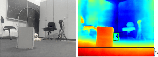
The depth estimation process outputs a depth map (also called a depth image or depth mask) of the same size as the RGB images it is associated with. 

And each pixel's intensity in the map (depth value) represents the distance to the corresponding point in the original scene. Typically, lighter pixels indicate closer objects, while darker pixels indicate objects farther away. 

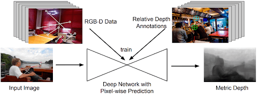
Practically, monocular depth estimation uses deep learning approaches to estimate depth. Since a single image contains no direct distance measurements, a neural network learn to recognize visual patterns that correlate with depth (monocular cues).

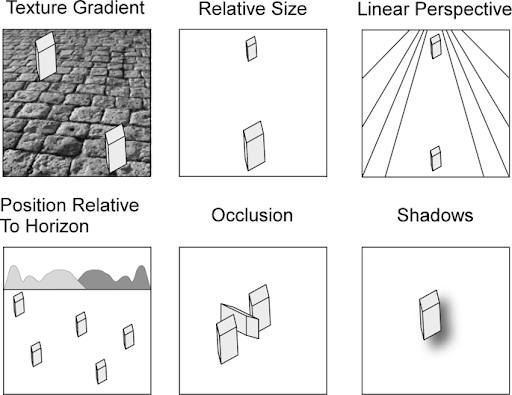
These cues are similar to those our brain uses to perceive 3D space, including:

• Perspective: Parallel lines appearing to converge in the distance.
• Object Size: Familiar objects look smaller when they are farther away.
• Texture Gradient: Textures appear finer and less detailed as they move into the distance.
• Occlusion: When one object partially blocks another, we know the blocking object is closer.

For example, when the model takes an image of a chessboard, it processes it and then produces a depth map (often normalized so that larger values indicate greater distance). 

In this map, the chess pieces in the foreground appear bright white, while those further back are shown in gradually darker shades of gray, with the most distant parts fading to nearly black. And it provides a detailed (pixel-level) understanding of the scene geometry.

When discussing depth estimation, it's important to distinguish between two main categories:

• Absolute Depth Estimation (Metric Depth): It aims to provide exact depth measurements from the camera. The term is used interchangeably with metric depth estimation (how far things are in real life), in which depth is measured in precise units, such as meters or feet. Absolute depth estimation models output depth maps with numerical values that represent real-world distances.
• Relative Depth Estimation: Predicts the depth order (magnitude) of objects or points in a scene without providing measurements. These models output a depth map that shows which parts of the scene are closer or farther (relative closeness) without actual distances to A and B.

Why Depth Estimation Matters (Applications and Use Cases)

Depth information is crucial for many vision tasks because depth maps enable us to go beyond 2D object recognition by turning a flat image into a 3D understanding. 

Here are some of the most common applications.

Autonomous Driving and Robotics

Depth information helps estimate distances to vehicles, plan paths, and avoid collisions in autonomous driving and robotics. 

Traditionally, they depended on costly sensors like LiDAR or stereo cameras to measure depth. But monocular depth estimation provides a more affordable alternative that can augment or even replace LiDAR. 

It can be the primary depth sensor in budget-conscious applications or act as a redundant safety system to other sensors and provide crucial distance data for live decision-making.

Augmented Reality (AR) and Virtual Reality (VR)

Monocular depth estimation improves AR and VR by enabling the natural placement of virtual objects in the real world on devices like smartphones and AR glasses. 

Depth maps ensure proper occlusion and make interactions between virtual and real objects seem more believable.

3D Reconstruction and Mapping

Monocular depth models can convert video or single photos into 3D models of a scene. It can be used for applications like interior scanning, cultural heritage preservation, and creating assets for virtual reality.

3D reconstruction is achieved by combining each pixel's 2D coordinates (x, y) with its predicted depth value (z) to create a 3D point (x, y, z) in space. When done for all pixels, this process generates a 3D point cloud of the scene geometry.

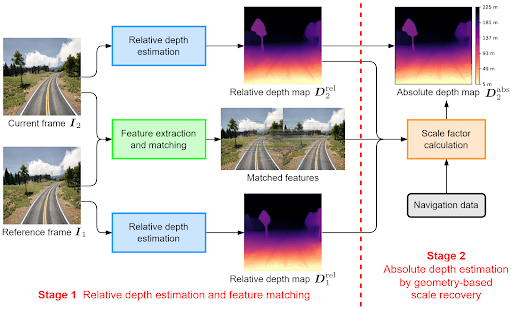
For example, this paper proposed the framework MURRe (Multi-view Reconstruction via SfM-guided Monocular Depth Estimation), which uses a multi-stage pipeline for 3D reconstruction.

• Structure from Motion (SfM): First, it analyzes multiple input images to create a sparse 3D point cloud (a structural skeleton).
• Guided Estimation: This sparse data guides a generative model (diffusion network) to produce a dense, highly detailed, and accurate depth map for each view.
• Fusion: Finally, all the refined, high-quality depth maps from the different views are fused into a single and clean 3D model of the scene.

MURRe individual depth predictions from various angles are combined to create a single 3D reconstruction of the environment (a collection of objects, an indoor room, or a large-scale cityscape).

Semantic Understanding and Object Detection

Depth maps improve semantic segmentation and object detection by providing a third dimension (a sense of how far away objects are).

For example, a simple object detection system can detect a car in an image and draw a box around it, and show the object's location and type (what and where in 2D). However, it doesn't know how far the car is from us or the scale.

Monocular depth estimation adds this information by estimating the distance to objects. 

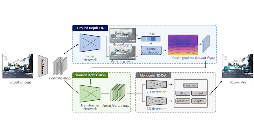
For example, using the 2D bounding box from an object detection model with the predicted depth value for that object, we can perform 3D object detection. It creates a 3D bounding box that describes the object's position and scale in the real world.

For any autonomous agent, this fusion of data is important, as in self-driving cars, which need to know whether a pedestrian is 10 meters or 100 meters away, since the required safety action is completely different.

Medical Imaging

Monocular depth estimation principles are also used in medicine. 

During minimally invasive surgeries, an endoscopic camera provides a single video feed from inside the body.

A depth model can analyze this feed to create a 3D map of organs and tissues. It then helps surgeons see better in 3D and makes it easier to navigate and perform surgeries accurately.

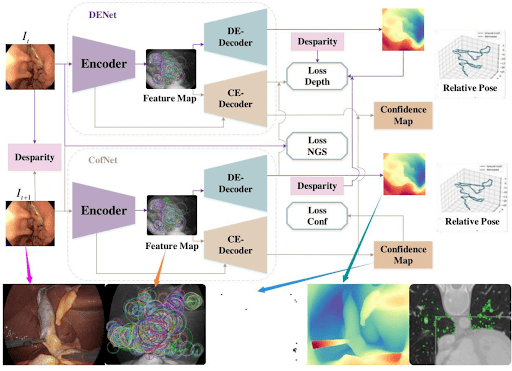
For example, the neural network takes endoscopic images as input and uses an encoder-decoder structure to extract feature maps.

From these features, the model generates a disparity (depth) map and a confidence map, which are used to reconstruct the 3D scene geometry of the internal anatomy in real-time. 

Challenges in Inferring Depth from a Single Image

Estimating depth from one image is difficult (ill-posed problem). Since no stereo parallax is available, the model has to rely on learned priors and visual cues. Key challenges include:

• Ambiguity and Lack of Direct Cues: A single image projection can correspond to infinitely many 3D scenes, which makes depth ambiguous. Shiny, transparent, or textureless surfaces confuse networks, since reflections or uniform areas carry little depth cues. For example, a white wall and a distant foggy landscape might look similar even though their distances differ greatly.

• No Stereo or Motion Parallax: Stereo or motion provides strong geometric cues (disparity or optical flow). Monocular methods lack those, so they must infer geometry purely from context, which can fail in novel scenes.

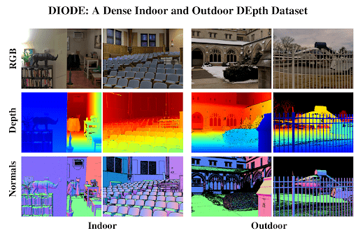
• Variety of Scenes (Generalization): A depth estimation model trained on a specific type of environment can struggle to generalize to unseen scenes. For example, a model trained on the DIODE dataset's indoor scenes might perform poorly on outdoor driving scenarios because the statistical patterns, lighting conditions, and object types are vastly different (domain shift).
  
  
• Need for Dense Ground Truth: Training a supervised depth model requires ground truth depth for every pixel of many training images (RGB-to-depth pairs). But capturing ground-truth depth, like with LiDAR or structured light, is costly. Also, unlike labeling classes for image classification, you cannot have a human hand-label a depth map.

• Real-Time and Resource Constraints: For many practical applications, such as mobile AR, the depth estimation model must run in real-time on hardware with limited computing power and memory. But, large SOTA accuracy neural architectures are often too slow for deployment on edge devices. Therefore, this creates a constant trade-off between model performance and efficiency.

Building and Training a Monocular Depth Estimation Model

Developing a monocular depth estimation model involves a thorough process that spans data collection, architecture design, training, and evaluation. 

Each step presents unique considerations that an ML engineer must address to build a powerful system.

Data Collection and Preparation

A good depth estimation model training starts with a high-quality, relevant dataset of RGB images paired with ground-truth depth maps. 

The data you choose depends on your use case, and there are many publicly available datasets you can utilize. 

So, let's go over some popular datasets.

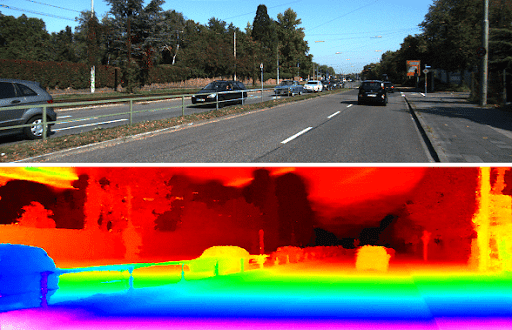
• KITTI (2012/2015): It is widely used to evaluate autonomous driving systems. KITTI contains outdoor driving scenes with 3D depth information from LiDAR sensors for thousands of road images (93,000 images for training). 

• Models trained on KITTI are good at estimating distances to objects on the road but might struggle with objects outside the LiDAR's field of view.

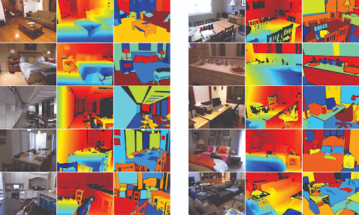
• NYU Depth V2: Indoor scenes (living rooms, offices, and kitchens) captured with a Microsoft Kinect sensor. It provides 1,449 densely labeled RGB-D image pairs (plus hundreds of thousands of unlabeled frames). 

• Depth values here are in meters (about 0-10 meters) and can fail on reflective or dark surfaces.

• DIODE (Dense Indoor/Outdoor DEpth): It covers both indoor and outdoor environments and contains thousands of high-resolution images with dense far-range depth.

• DIODE is unique in covering both domains with one sensor suite. It offers a depth accuracy of ±1 mm for indoor use and up to 350 meters for outdoor applications.

• MegaDepth: A large-scale dataset derived from internet photo collections using Structure-from-Motion and Multi-View Stereo (SfM/MVS). 

• MegaDepth provides dense depth maps and corresponding RGB images and enables single-image depth learning with broad scene variety.

• DIW (Depth in the Wild): It contains unconstrained Internet images annotated with relative depth (ordinal pairs). And it helps models learn depth ordering even when metric depth is unavailable.

• Synthetic datasets (Sintel, FallingThings): Datasets such as FallingThings (FAT), Virtual KITTI, or Scene Flow that simulate depth from graphics engines. 

Pro tip: Check our Guide to Synthetic Data Generation (And How Lightly Can Help)

• For example, FallingThings (FAT) includes 60k synthetic scenes with mono/stereo RGB, dense depth, 3D poses, segmentation, and bounding boxes.

Most of these datasets typically come as PNG or JPG image formats and depth maps (often 16-bit PNGs or NumPy arrays). So it’s important to align the depth maps with the images (same width/height and camera parameters). 

All the above-mentioned datasets can be used in the first place. 

But if you want a depth estimation model that can understand your domain. Then you need your domain data and perform depth annotation with some software or methods (if LiDAR is costly). 

Pro tip: If you are looking for the perfect data annotation tool or service, make sure to check out our list of 12 Best Data Annotation Tools for Computer Vision (Free & Paid) and  5 Best Data Annotation Companies in 2025.

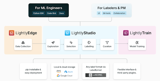
To collect domain data, you can use LightlyEdge. It is a smart data selection SDK that runs on edge devices (data collection devices). It analyzes incoming data in real-time and only collects the most valuable and informative frames that match your individual criteria, like the Scene of interest.

After collecting the data, you can use LightlyStudio for further curation and labeling. It can help select a diverse, high-quality subset from large image collections. 

LightlyStudio ensures that when you send data for depth annotation, you focus on samples that actually improve model generalization.

If you like code, then access LightlyStudio Python SDK and API support, and build on open-source standards designed for flexibility and scale.

Now, let's understand the model architectures.

Model Architecture

Monocular depth models are typically encoder–decoder neural networks. 

This two-part architecture nicely turns a high-resolution input image into a dense, pixel-aligned depth map.

The encoder is usually a Convolutional Neural Network (CNN) that processes the input image to extract a rich set of feature maps. It learns to recognize an implicit relation between color pixels and depth (capturing semantic and geometric cues). 

Since building and training a CNNs encoder from scratch is difficult, we usually use a pretrained backbone (ResNet or DenseNet). They trained on a general dataset, but with transfer learning, we make it work for our more specific use case.

And the decoder then takes these compact features and intelligently upsamples them, often using skip connections to reintroduce fine details from the encoder, to reconstruct the final, full-resolution depth map image.

However, modern approaches add sophistication, for instance, transformers or self-attention blocks for global scene understanding, or multi-scale fusion. 

For example, AdaBins use a CNN backbone plus a transformer-based “adaptive binning” module that divides depth values into learned bins and allows more precise predictions.

Similarly, models like DPT (Dense Prediction Transformer) perform pixel-based analysis to analyze the entire scene context at once.

The self-attention block in transformers allows the depth model to have a higher capacity interpretation of scene geometry and improves ambiguity resolution.

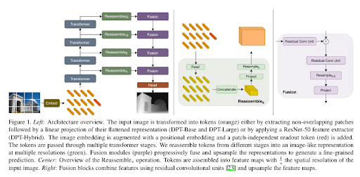
Methods like DPT work well with supervised learning and depend on large, labeled datasets (ground truth), which are expensive, time-consuming, and can have biases.

These limitations can be overcome using unsupervised and self-supervised learning for monocular depth estimation.

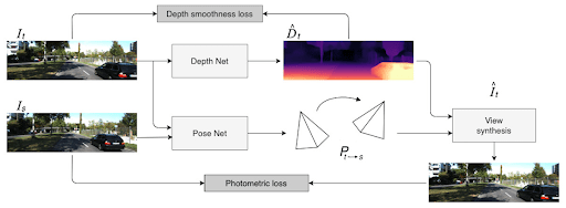
Self-supervised learning uses the data itself as the supervision signal (guidance). The key task of the model is to predict depth maps from images (or stereo pairs), without requiring expensive ground-truth depth labels. 

A depth network and a pose network are jointly trained to reconstruct target views from source views using photometric consistency (reprojection loss + image similarity).

The architecture choice also depends on the use case. For example, if you're planning to run the model on mobile devices, then lightweight neural networks such as DepthNet and MobileNet-based are good options. 

On the other hand, heavy transformer models require GPUs to get top accuracy on benchmarks. 

The Training Process

After the data and model are prepared, we start teaching the model to make accurate predictions. It's an iterative loop guided by a loss function, which measures the error between the model’s depth prediction and the ground truth. 

Common supervised loss choices include:

• Pixel-wise Losses: L1 (Mean Absolute Error) and L2 (Mean Squared Error) losses compute the average per-pixel difference between the predicted and true depth. Often depth is in meters, so these losses directly penalize distance errors. 
• Scale-Invariant Loss:  A common approach is to use the Scale-Invariant Logarithmic Error (SI-log) to train models for relative depth. It penalizes errors in the relationships between pixel depths rather than their absolute values. It is often computed as the L2 norm of the difference between the logarithms of the predicted and true depth values.
• BerHu (Reverse Huber) Loss: It's a hybrid loss that behaves like an L2 loss for small errors and an L1 loss for large errors, combining the benefits of both.   
• Multi-scale Loss: Depth may be predicted at multiple scales, so losses (choice of loss function) are applied at each scale to capture coarse and fine errors.

Furthermore, in a self-supervised setting where no ground-truth depth is available, the main guide is the photometric reconstruction error. Here, the model predicts a depth map from one image and uses it to "warp" that image to a neighboring viewpoint (from a video or stereo pair). 

The loss is the difference (typically a mix of L1 and SSIM) between this synthesized image and the actual target image. 

Similarly, unsupervised methods (including self-supervised) add a smoothness loss to encourage local gradients (since depth should be piecewise smooth). 

The calculated error loss is then fed to an optimizer, such as Adam, which uses this signal to adjust the model's weights. This process is fine-tuned by hyperparameters like the learning rate (how big a step the optimizer takes), the number of epochs, and the batch size. 

Throughout training, the model's performance is monitored on a separate validation set to check for overfitting and determine when the model has learned effectively.

Sometimes, the model's raw output can be slightly noisy. To avoid this, you can apply post-processing filters, such as a bilateral filter, to the predicted depth map to smooth out imperfections while preserving sharp edges.

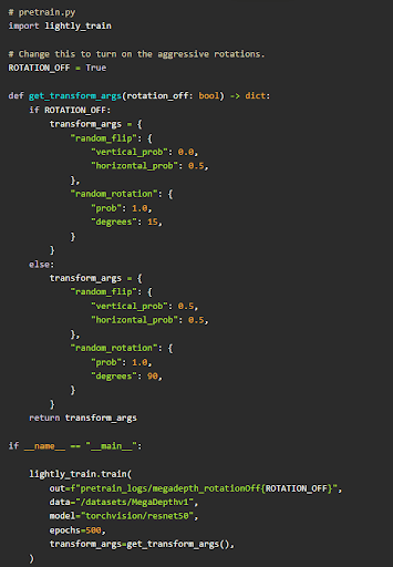
Another way to overcome this for visual improvement is to pretrain the model before fine-tuning. With LightlyTrain, pretraining is as easy as writing a few lines. 

See the sample code below. For an end-to-end implementation of monocular depth estimation with fastai U-Net + LightlyTrain, check it out here. 

Evaluating and Refining the Output

After training is complete, the model's final performance is measured on a hidden test set. We use specific evaluation metrics to quantify its accuracy. 

Common evaluation metrics include:

• Abs Rel (Absolute Relative Error): It is the mean of the absolute relative error between predicted and ground-truth values. This tells, on average, how off the prediction is relative to true depth (good for metric depth).

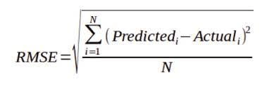
• RMSE (Root Mean Squared Error): RMSE is the square root of the average squared difference between predicted and ground-truth values. Often measured in the dataset’s depth units (meters). There’s also RMSE(log) for log-depth errors.

• Relative ranking metrics: For relative depth tasks or datasets like DIW, sometimes WHDR (Weighted Human Disagreement Rate) is used.

Step-by-Step Example: Implementing Monocular Depth Estimation

Depth models accessed through platforms like PyTorch Hub have made it much simpler for us to get started and get great results with pre-trained models. 

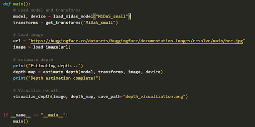
So, let's write some code and perform inference using the MiDaS model. 

First, we define functions to load the pre-trained MiDaS model from the PyTorch Hub and set it to evaluation mode. The transform function prepares the image by resizing and normalizing it to the model's expected input format.

Next, we need a function to load an image from either a URL or a local file path. The load_image function ensures the image is in RGB format, which the model requires.

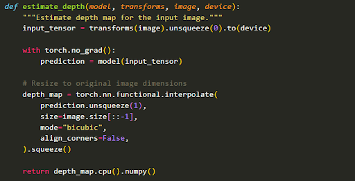
Now, the function below (estimate_depth) takes the loaded model, the transforms, and the image to perform the depth estimation, then resizes the output depth map back to the original image's dimensions.

Here, we create functions to normalize and visualize the depth map to interpret the model's output. 

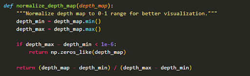
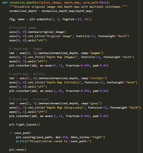
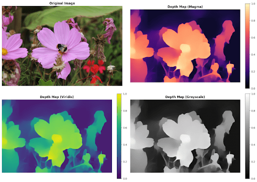
We will display the original image alongside the depth map rendered with various colormaps (Magma, Viridis, and Grayscale) to highlight different depth details with the function below.

‍

Now we are all good with the function. Finally, a main function combines the entire process, calling each helper function in sequence to go from a source image URL to a final visualization.

Output:

State-of-the-Art Models and Performance Comparison

Monocular depth estimation has seen rapid progress, with methods and training approaches constantly pushing the limits of performance. The table below compares several landmark models.

‍

Simply put, monocular depth models are now usable for many tasks. But you must choose the right model for the job, a fast, lightweight model for real-time on-device use vs. a heavy, accurate model for offline processing. 

How Lightly AI Accelerates Depth Estimation Model Development

Training robust depth estimation models needs extensive data to account for diverse lighting, weather, and complex scene geometry.

But collecting and then labeling this data is inefficient. Much of it, like repetitive driving footage, is redundant and adds little value to the model while driving up costs.

This is where Lightly AI's platform steps in to address the data bottleneck and provides tools for developing high-accuracy depth models while minimizing costs and effort

• LightlyEdge helps you gather your domain-specific data without collecting duplicate images. You can use different devices to collect the dataset based on set criteria, and the SDK runs directly on these devices.

• LightlyStudio then uses active learning to analyze your large pools of raw, unlabeled domain-specific images (collected from LightlyEdge or any other source). And it helps automatically select the most informative, diverse subsets for labeling (depth annotation). It can prioritize edge cases (unusual lighting, rare viewpoints) where models typically struggle, reduce labeling needs, and accelerate your model's path to better generalization.

• LightlyTrain then enables self-supervised pretraining, training your own vision models on this unlabeled data using state-of-the-art SSL methods, so that feature extraction is adapted to your data domain. This pretraining enhances depth inference from monocular cues and speeds up convergence for downstream tasks (absolute or relative depth prediction).
  
  
• Lightly AI Data Services for GenAI extend these capabilities beyond vision. Through expert-led data curation, prompt evaluation, bias detection, and data quality audits, the GenAI data services team helps organizations refine and scale datasets for multimodal and language model applications, ensuring models learn from high-quality, representative data that generalizes well to real-world use cases.

The best part is that LightlyEdge + LightlyTrain easily integrates with LightlyStudio. Data intelligently captured by Edge can be fed into Studio for quality assurance and further curation. 

Then, Trian can pretrain the model using that unlabeled data. They create an end-to-end pipeline for building better datasets and models with less effort.

Conclusion

Monocular depth estimation turns a flat RGB image into 3D scene understanding. Despite their challenges, advances in neural networks and large-scale training have yielded impressive results. 

Also, depth estimation merges with other vision tasks and lets models learn depth, semantics, and geometry jointly. 

By following best practices in data preparation and training, using the latest models and data curation tools, ML engineers can create systems that bring depth awareness to any single-camera app.