Diffusion Transformers Explained: The Beginner’s Guide
Table of contents
Share blog post


Diffusion Transformers (DiTs) replace U-Nets with Vision Transformers in diffusion models, operating in latent space for efficient, high-quality generation. They scale well, power state-of-the-art models, and are used in systems like SORA and Stable Diffusion 3.
Share blog post
The answer to some common questions about Diffusion Transformers:
- What are Diffusion Transformers?
Diffusion Transformers (DiTs) are a new class of generative models that combine diffusion models with a Transformer architecture. They replace the commonly used U-Net backbone in diffusion models with a transformer network, operating on latent space representations instead of pixel space.
This allows the model to leverage self-attention for capturing global context during the image diffusion process.
- How do Diffusion Transformers differ from traditional diffusion models?
Unlike prior diffusion models which use convolutional U-Net networks, DiTs use Vision Transformer blocks as the denoising model.
The transformer processes latent patches of the image (produced by a VAE encoder) as a sequence of input tokens, with positional embeddings just like in ViT. This architecture introduces no inherent spatial bias, showing that the U-Net’s inductive bias (local convolutional structure) is not strictly necessary for high-quality image generation.
- Why use Transformers in diffusion models?
Transformers offer good scalability properties – as you increase model depth/width or the number of input tokens, generation quality improves (measured by FID).
DiTs have demonstrated state-of-the-art image quality on benchmarks (e.g. ImageNet) while being more compute-efficient than pixel-space U-Nets.
- What is DiT-XL/2 and why is it important?
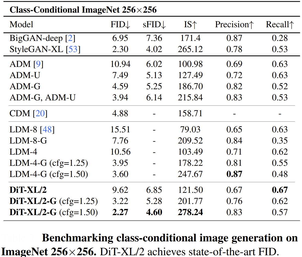
DiT-XL/2 refers to the largest Diffusion Transformer model configuration introduced by Peebles & Xie (2023). “XL/2” denotes an Extra-Large model using a patch size of 2 (meaning smaller patches, more tokens). This model (with ~675M parameters) achieved state-of-the-art FID scores (e.g., 2.27 on ImageNet 256×256) that outperform all prior diffusion models.
Despite its high complexity (~119 GFlops per forward pass), it’s still more computationally efficient than previous pixel-space models, thanks to operating in a lower-dimensional latent space. DiT-XL/2’s success proved that scaling model size and tokens in a transformer-based diffusion model can push image generation to new quality levels.
- Are Diffusion Transformers used in current AI models?
Yes – the Diffusion Transformer model has inspired several cutting-edge systems. For example, OpenAI’s SORA video generator uses a diffusion transformer to produce high-fidelity videos from text prompts.
Stability AI’s upcoming Stable Diffusion 3 incorporates a diffusion transformer architecture (combined with a flow-matching technique) to improve text-to-image generation. Research models like PixArt-α are purely transformer-based diffusion models for text-to-image synthesis, achieving quality on par with Stable Diffusion and Midjourney while training much faster.
Introduction
What if the same transformers that mastered language could master images too?
Enter Diffusion Transformers, the engine behind the next wave of creative AI.
It’s 2025, and Generative AI has advanced rapidly, with diffusion models leading the way in producing high-quality images, videos, and more. Traditionally, these models have relied on U-Net architectures to gradually refine noisy inputs into realistic outputs.
However, a new approach is reshaping the field: Diffusion Transformers (DiTs).
By replacing the U-Net backbone with a Transformer architecture, DiTs bring the scalability, global context modeling, and flexibility of transformers into the diffusion process.
Here’s what we will cover in this article:
- Background Recap of Transformers and Diffusion Models
- Diffusion Transformers: What they are, and how they are different
- Architecture Details of DiTs
- Training of DiTs
- Scalability and Performance of DiTs
- Applications and State-of-the-art Developments
Training Diffusion Transformers effectively depends on both high-quality data and efficient pretraining strategies. At Lightly, we help you get the most out of your generative workflows with:
- LightlyTrain: Pretrain and fine-tune vision backbones for Diffusion Transformers to speed up convergence and improve sample quality.
- LightlyOne: Curate diverse, high-impact data to reduce redundancy and ensure your models learn from the most informative examples.
Together, they help you build better, faster, and more efficient generative models for images, video, and beyond.
See Lightly in Action
Curate and label data, fine-tune foundation models — all in one platform.
Book a Demo
Background: Transformer Diffusion Models and Basics
Before we dive into Diffusion Transformers, let’s recap our understanding of Transformers and Diffusion models.
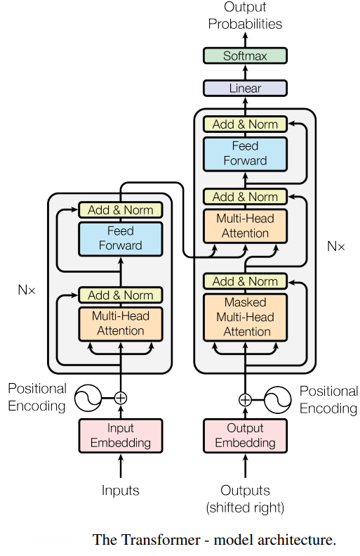
Transformer Basics: The Architecture That Changed Deep Learning
Transformers (introduced by Google in the revolutionary “Attention is All You Need” paper) have radically transformed how machines understand data, laying the groundwork for breakthroughs in language, vision, and multimodal AI.
At their core, transformers introduce a novel way of processing information: rather than handling data in sequence, they rely on self-attention, an ability to weigh and relate all pieces of input simultaneously.
This shift from stepwise computation to parallel reasoning enables models to grasp long-range relationships and contextual nuances with remarkable efficiency.
The Heart of Transformers: Attention Mechanism
What truly powers transformers is their attention mechanism.
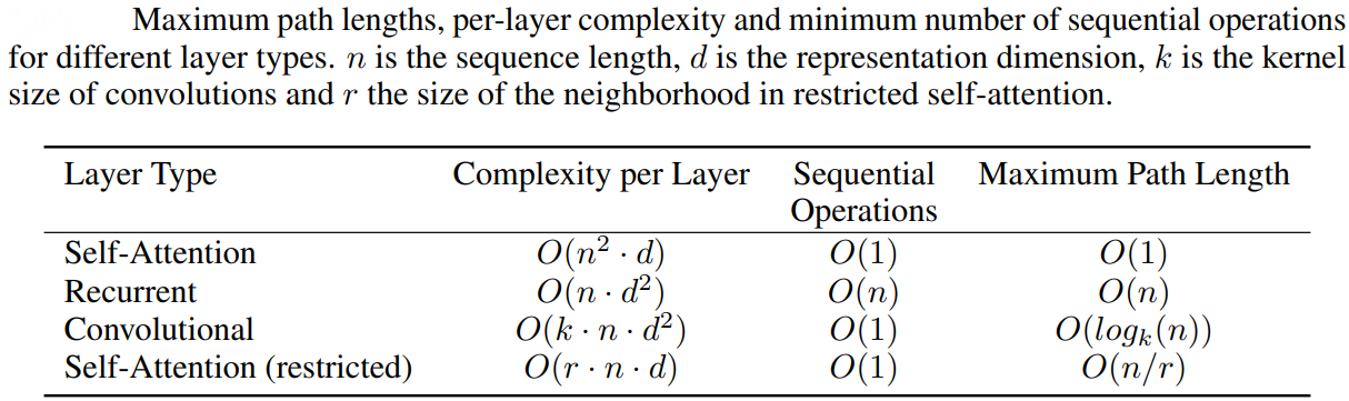
Traditional neural networks, like RNNs and CNNs, focus on local or sequential patterns, but transformers revolutionized deep learning with the attention mechanism. Attention lets the model evaluate the importance of every input token with respect to every other token, regardless of their position or proximity.
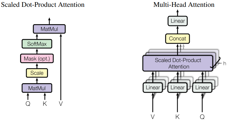
The attention mechanism is built on three fundamental components: Query, Key, and Value vectors. For each input token (be it a word in a sentence or a patch of an image), the model computes these vectors:
- Query (Q): Represents the current token's "question"—what it wants to know about its context.
- Key (K): Encodes each token's "identity" or features, effectively acting as what other tokens broadcast about themselves.
- Value (V): Carries the actual information each token contributes to the output.
The attention score for each token pair is computed as a dot product between Q and K vectors, scaled and passed through a softmax to produce weights. These weights then determine how much each token's Value influences the final representation:
Attention(Q, K, V)=softmax(QKTdk)V
Here, dk is the dimensionality of the Key vectors, serving as a scaling factor. This mechanism lets transformers dynamically focus on the most relevant parts of the input, aggregating global context at every layer.
Self-Attention: Modeling Global Context
Self-attention is the main ingredient behind a transformer's ability to capture context and relationships across long distances in data.
- How it works: For a sequence of tokens (such as words or image patches), each token’s Q vector interacts with all K vectors in the same sequence, calculating how much each token should "attend to" the others.
- The resulting attention weights let the model form contextualized representations, where each token’s meaning can depend on distant interactions, resolving ambiguities and nuanced dependencies.
Example: In a sentence, self-attention allows “it” to relate to the correct antecedent, regardless of their separation.
Multi-Head Attention: Diversity in Focus
To further enhance flexibility, transformers use multi-head attention. Instead of a single attention calculation, the mechanism runs several in parallel, each called an “attention head.”
- Each head has its own set of learned weight matrices, projecting Q, K, V into distinct subspaces.
- Independent attention scores are calculated for each head, capturing varying relationships (e.g., syntactic, semantic, spatial).
- The outputs of all heads are concatenated and linearly transformed, giving a richer, multi-faceted understanding at every layer.
This parallelism lets transformers simultaneously attend to different types of patterns, crucial for tasks involving layered meaning or multiple objects.
Self-Attention vs. Cross-Attention
While self-attention connects parts within a single input (such as a sentence or an image), cross-attention bridges between different sequences.
- Self-attention: Query, Key, and Value vectors come from the same sequence, enabling internal context modeling.
- Cross-attention: Typically used in encoder-decoder models; Queries come from the decoder’s state, while Keys and Values come from the encoder’s output. This allows the decoder, say, in language translation or text-to-image synthesis, to pull pertinent information from the encoded input as needed.
Example: In a text-to-image model, cross-attention helps the image generator focus on relevant parts of the text prompt at each step.
Other important architectural components
The other important architectural components that make transformers work for NLP or vision tasks are:
- Positional Embeddings: Transformers process tokens in parallel, but sequences like text and images have order and structure. To retain this information, positional embeddings are added to input vectors, injecting location awareness and allowing the model to differentiate, for example, between the start and end of a sentence or rows and columns in an image.
- Building Blocks and Scalability: Transformers stack layers of multi-head self-attention, feedforward networks, and normalization, creating deep models that scale efficiently. This scalability, along with their ability to manage vast amounts of context and learn diverse patterns, is why transformers dominate modern AI, and why their use in diffusion models has sparked the recent wave of breakthroughs in generative technology.
By leveraging these mechanisms, transformers set a new standard for flexibility, compositional understanding, and performance in deep learning- capabilities that are now being harnessed by Diffusion Transformers in state-of-the-art generative tasks.
Diffusion Models Basics: The Foundation of Modern Generative AI
Diffusion models have risen to prominence as one of the most powerful approaches for generating realistic images, audio, and more. Their success comes from a unique process that incrementally refines noisy data into coherent outputs, guided by learned patterns from vast training sets.
At the heart of diffusion models is a simple yet profound idea: teaching the model to reverse a gradual noise process.
Instead of generating images in a single step, diffusion starts with pure noise and then removes small amounts of noise over many steps to reveal structured content.
- Forward process: The real image is repeatedly corrupted with noise, eventually turning it into pure noise. Each step adds a little noise according to a predefined schedule.
- Reverse process: During generation, the model is trained to denoise these corrupted images, step by step, until a clean, realistic image emerges.
How Diffusion Models work
The step-by-step nature of the diffusion process is formally described using a Markov chain.
A Markov chain is a mathematical model for a sequence of events where the probability of transitioning to the next state depends only on the current state, not on the sequence of states that preceded it. This is often called the "memoryless" property. Think of it like a board game: your next possible move is determined solely by the square you are on right now, not by the path you took to get there.
In diffusion models, this simplifies the math immensely:
- The noisy image at timestep t is generated directly from the image at timestep t-1.
- To know the state of xt, you only need to know xt-1, not the original clean image or any other intermediate steps.
- Given an image x0, noisy versions x1,x2,..., xT, are formed with increasing noise at each timestep.
This structure allows the forward process to be defined as a series of simple transitions where Gaussian noise is added at each step:
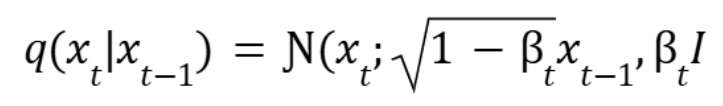
Here, βt is a small positive constant that controls the amount of noise added at each step t.
The model's goal is to learn the reverse of this process: how to transition from a noisy state back to a cleaner one, step by step, until a realistic image is formed.
The denoising model (often a U-Net or, with DiTs, a transformer) learns to estimate either the clean image or the added noise at each step, so that it can iteratively recover x0 from xT. The typical objective is a reconstruction or denoising loss (often mean squared error) between the predicted and true noise. Some advanced variants model the probability of entire trajectories, making the process more data-efficient and robust.
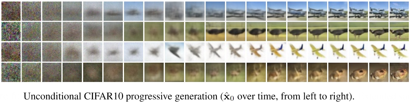
Generating a new sample with a diffusion model involves iteratively applying the learned denoising steps to a starting noise tensor. Each step reduces randomness and increases structure, guided by the model’s predictions:
- Start with random noise xT.
- Use the model to predict clean image or noise.
- Gradually step towards less noisy images xT-1, xT-2, ..., x0.
- The process yields a high-fidelity, realistic output.
Diffusion models are highly flexible and can be conditioned to produce images from text prompts, generate audio from waveforms, or synthesize data with specified properties. Conditioning is typically achieved by feeding auxiliary inputs (like embeddings) into the denoising model.
StableDiffusion is the first diffusion model to revolutionize the generative AI technologies, which performs the diffusion process (noise addition and removal) in the latent space (i.e., on the embeddings of images) instead of in the pixel space (raw images).
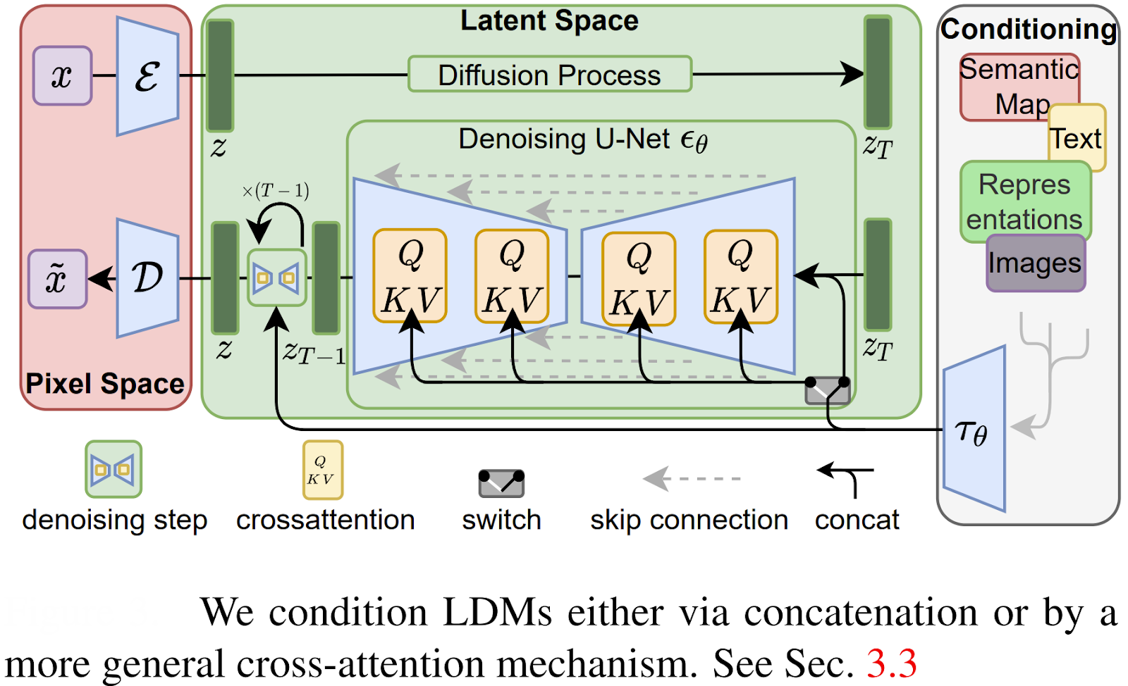
Latent diffusion is better than pixel space diffusion and thus has become more widely adopted because of the following:
- Computational Efficiency: By performing the diffusion process on compact latent representations instead of raw pixels, latent diffusion models require far less computational power. This significantly speeds up the overall generation process and makes it feasible to run on consumer-grade hardware.
- Scalability to High Resolutions: Working in a compressed latent space makes it easier to generate high-resolution images without a proportional increase in computational cost.
- Faster Processing: The model can process millions of fewer values (latent vectors vs. pixels) during each step of the diffusion process, resulting in faster image creation.
- Improved Control: The latent space often captures semantically meaningful patterns (like object shapes and textures) more effectively, which can be leveraged for more precise control over the generated content.
- Flexibility for Conditioning: Latent diffusion models can be easily conditioned on various inputs, such as text prompts, to guide the generation process and enable tasks like text-to-image synthesis.
Diffusion Transformers: A New Class of Diffusion Models
Now that we’ve covered the fundamentals of both diffusion models and transformers, we can explore what happens when these two powerhouse technologies are combined: Diffusion Transformers (DiTs).
Diffusion Transformers (DITs) is a groundbreaking architecture that reimagines the core of the diffusion process by replacing the traditional U-Net backbone, long the standard in diffusion models, with a pure Transformer network.

For years, the U-Net's convolutional structure was considered essential for image generation due to its strong inductive bias for spatial locality. It was believed this architecture was uniquely suited for processing pixel-level information.
Diffusion Transformers challenge this long-held assumption. By operating on a sequence of latent patches, compact representations of an image, instead of raw pixels, DiTs effectively apply a Transformer's core strengths to the denoising task. This allows the model to leverage self-attention to capture global context across the entire image at every step, a feat less natural for locally-focused convolutional networks.
The primary motivation behind this architectural shift is scalability. Transformers are famous for their remarkable ability to improve with size; as you increase their depth, width, or the number of input tokens, their performance consistently gets better. DiTs inherit this property, leading to a new generation of diffusion models that not only achieve state-of-the-art sample quality but also exhibit greater computational efficiency by operating in a lower-dimensional latent space.
In essence, DiTs prove that the U-Net's specific biases are not a prerequisite for high-fidelity image synthesis. Instead, a more general, scalable architecture can achieve even better results, paving the way for the next evolution in generative AI.
Now, let's look closer at how these models are constructed.
Architecture Details: Inside a Diffusion Transformer Model
To appreciate why DiTs are so effective, we need to look under the hood.
Their design cleverly combines a few key components to create a pure, transformer-based denoising engine that is both powerful and scalable. Unlike the intricate, multi-scale paths of a U-Net, the DiT architecture is remarkably straightforward.
1. Operating in Latent Space: The VAE Encoder/Decoder
The first crucial design choice is that DiTs do not operate directly on high-resolution pixel images. Doing so would create an impractically long sequence of tokens for a transformer to process. Instead, DiTs work in a compressed latent space.
- VAE Encoder: Before the diffusion process begins, a pre-trained Variational Autoencoder (VAE) encoder takes a high-resolution image and compresses it into a much smaller, lower-dimensional latent representation. This latent "image" captures the essential semantic information of the original image but is far more computationally manageable.
- VAE Decoder: After the transformer has finished its denoising work in the latent space, the VAE decoder is used to upscale the final latent representation back into a full-resolution pixel image.
This approach significantly reduces the computational load, allowing the transformer to focus its power on the core denoising task.
2. From Latent Image to a Sequence of Tokens
Transformers are designed to process sequences of tokens, like words in a sentence.
To make the latent image compatible, it is broken down into a sequence of smaller pieces:
- Patching: The latent image is divided into a grid of non-overlapping patches.
- Tokens: Each patch is then flattened into a vector. This sequence of vectors becomes the input for the transformer. In a DiT, image patches serve as tokens.
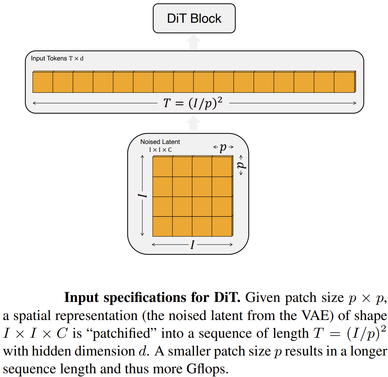
- Positional Embeddings: Since transformers process tokens in parallel, they have no inherent sense of order. To preserve the spatial structure of the image, positional embeddings are added to each patch token. These embeddings provide the model with information about the original location (row and column) of each patch in the grid.
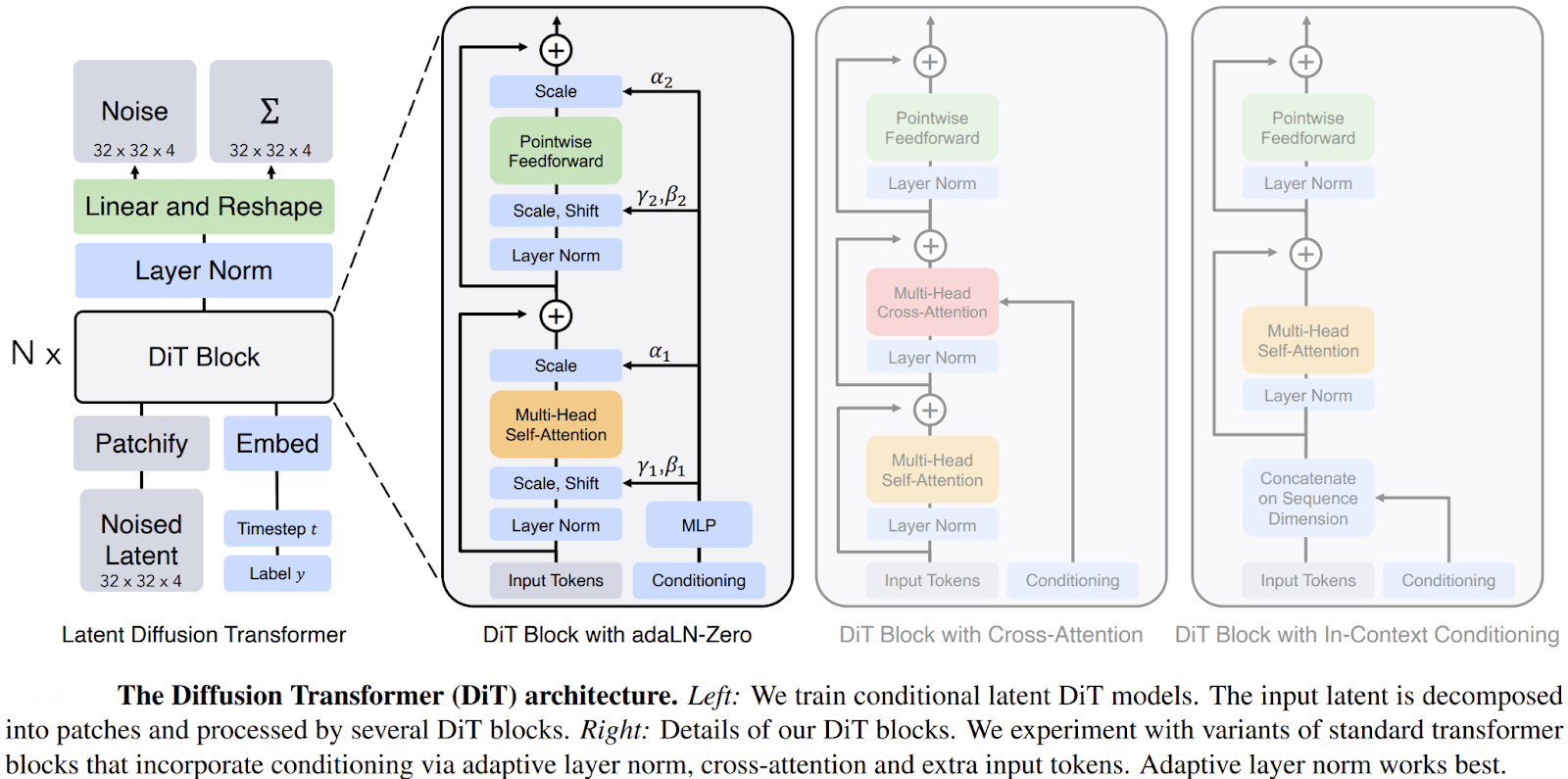
3. The DiT Block: A Vision Transformer for Denoising
The core of the model is a series of DiT blocks, which are based on the standard architecture of a Vision Transformer (ViT). Each block applies a series of operations to the sequence of patch tokens:
- Layer Normalization: Stabilizes the inputs to the block.
- Multi-Head Self-Attention: This is where the magic happens. The model calculates attention scores across all patch tokens, allowing it to capture global relationships and long-range dependencies across the entire latent image. Another layer normalization is added after this step for stability.
- Feedforward Network: A simple Multi-Layer Perceptron (MLP) processes each token independently, adding computational depth.
These blocks are stacked one after another to form the deep transformer network.
4. Conditioning: Guiding the Denoising Process
A diffusion model needs to know which denoising step it is on (the timestep t) and, for tasks like text-to-image, what content it should be generating (the text prompt or class label). DiTs incorporate this conditioning information in a particularly elegant way using adaptive Layer Normalization (adaLN).
Instead of simply concatenating the conditioning vectors (for timestep, class, etc.) to the input tokens, they are first processed by an MLP to produce scale (γ) and shift (β) parameters. These parameters are then used to modulate the activations within each DiT block, right after the Layer Normalization step. This allows the conditioning information to dynamically influence the entire network's computations at every layer, providing powerful and fine-grained control over the generation process.
By combining these elements, the DiT architecture successfully translates the denoising task of a diffusion model into a sequence-to-sequence problem perfectly suited for a transformer. This clean, scalable design discards the need for convolutional inductive biases and unlocks the full potential of transformer scaling laws for generative modeling.
Training Diffusion Transformers
Training a DiT follows the well-established paradigm of diffusion models, but with specific adaptations tailored to its unique architecture.
The goal is simple: teach the transformer network to accurately predict the noise that was added to a clean image’s latent at any given step in the forward diffusion process.
The training loop for a DiT can be broken down into a few key steps:
- Start with a Clean Image: A sample image is drawn from the training dataset (e.g., ImageNet).
- Encode to Latent Space: This image is passed through the pre-trained and frozen VAE encoder. This transforms the high-resolution image into a compact latent representation, z0. Freezing the VAE is a critical detail; it means the DiT model does not need to learn how to represent images, only how to denoise their latent forms.
- Apply Forward Diffusion: A random timestep, t, is selected from the full range of diffusion steps (e.g., from 1 to 1,000). The corresponding amount of Gaussian noise, determined by a predefined noise schedule, is added to the clean latent z0 to create a noisy latent zt. The actual noise vector used () is stored for the loss calculation.
- Predict the Noise: The noisy latent, zt is patched, positionally embedded, and fed into the Diffusion Transformer as a sequence of tokens. The model is also given the timestep t and any optional conditioning information (like a class label for class-conditional models, or a text prompt). The transformer processes this input and outputs a prediction of the noise, (zt,t).
- Calculate the Loss: The training objective is straightforward. The model's performance is measured by calculating the difference between the noise it predicted and the actual noise that was added in step 3. This is typically done using a simple Mean Squared Error (MSE) loss (E denotes expectation):
L=Ezo, , t[||-(zt,t)||2]
- Update the Model: The loss is backpropagated through the network to update the weights of the DiT. The process is then repeated with a new image and a new random timestep.
A key architectural element that plays a role in training is the adaLN mechanism. Instead of simply feeding the timestep and class embeddings into the model as extra tokens, they are used to dynamically adjust the activations within each DiT block. This ensures that the conditioning information effectively guides the denoising process at every level of the network, leading to more precise and controllable generation.
By repeatedly performing these steps on millions of images, the DiT learns a robust model of the data distribution, becoming highly proficient at reversing the diffusion process from any noisy starting point. This seemingly simple training scheme, when applied to a scalable transformer architecture, is what enables DiTs to achieve their state-of-the-art results.
💡Pro tip: Since training DiTs relies heavily on loss functions like MSE, you might want to explore our Guide to PyTorch Loss Functions to better understand how different loss choices affect model convergence and generation quality.
Scalability and Performance of Diffusion Transformers
The primary motivation for developing DiTs was to harness the proven scalability of the transformer architecture. In deep learning, a model is considered scalable if its performance reliably improves as more computational resources, data, or parameters are added.
The original DiT paper provides compelling evidence that DiTs not only inherit this property but thrive on it, setting a new standard for generative model performance.
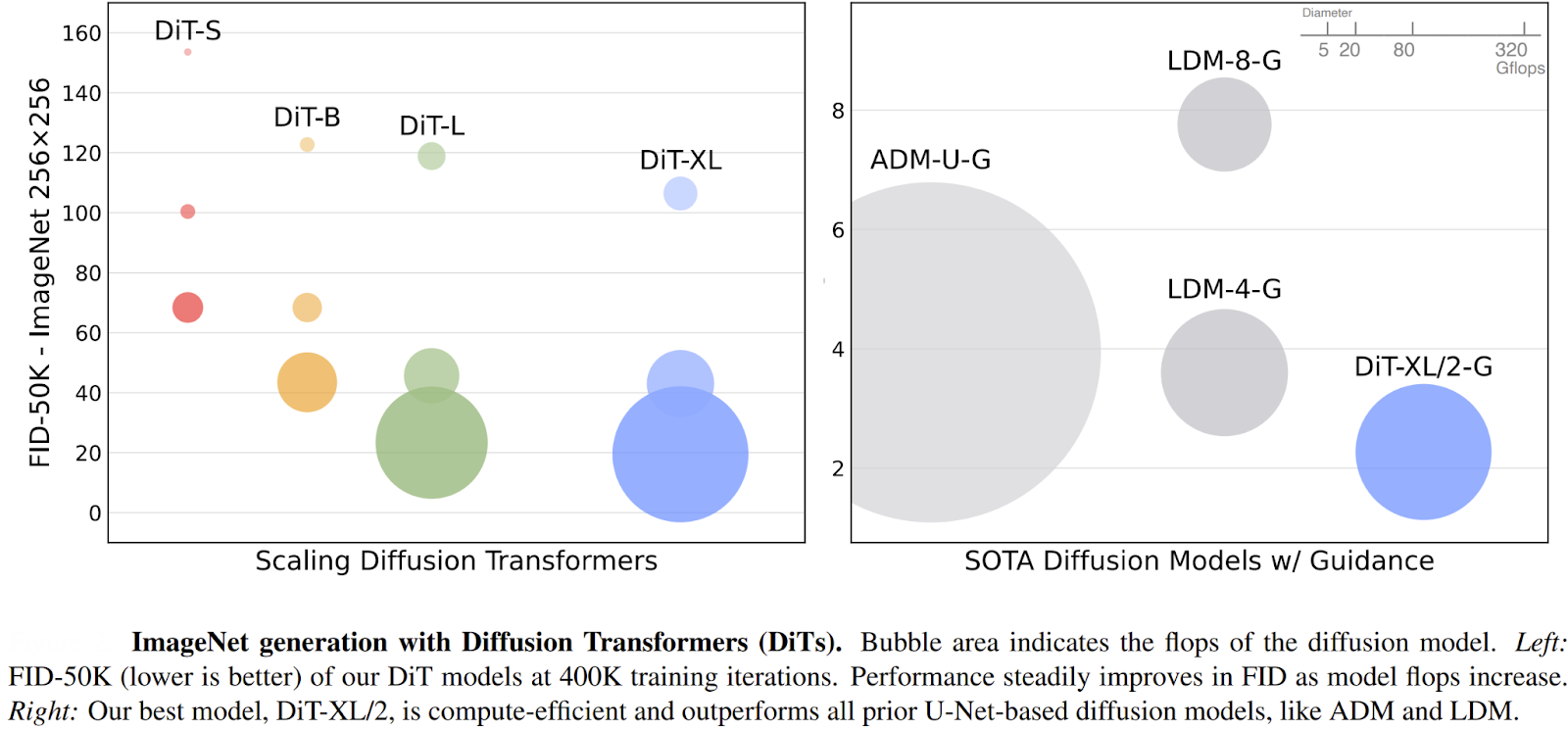
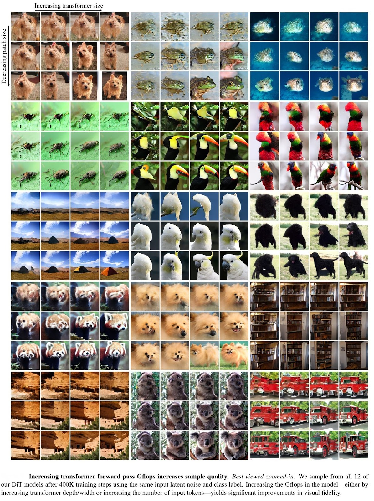
The authors analyzed the scalability of DiTs by measuring model complexity against sample quality (as shown above).
- Model Complexity was measured in Gflops (Giga Floating-Point Operations Per Second), which quantifies the total computational cost of a single forward pass through the network. A higher Gflops value indicates a more powerful, and computationally expensive, model.
- Sample Quality was evaluated using the Fréchet Inception Distance (FID), a standard metric where a lower score indicates that the generated images are more similar to real images.
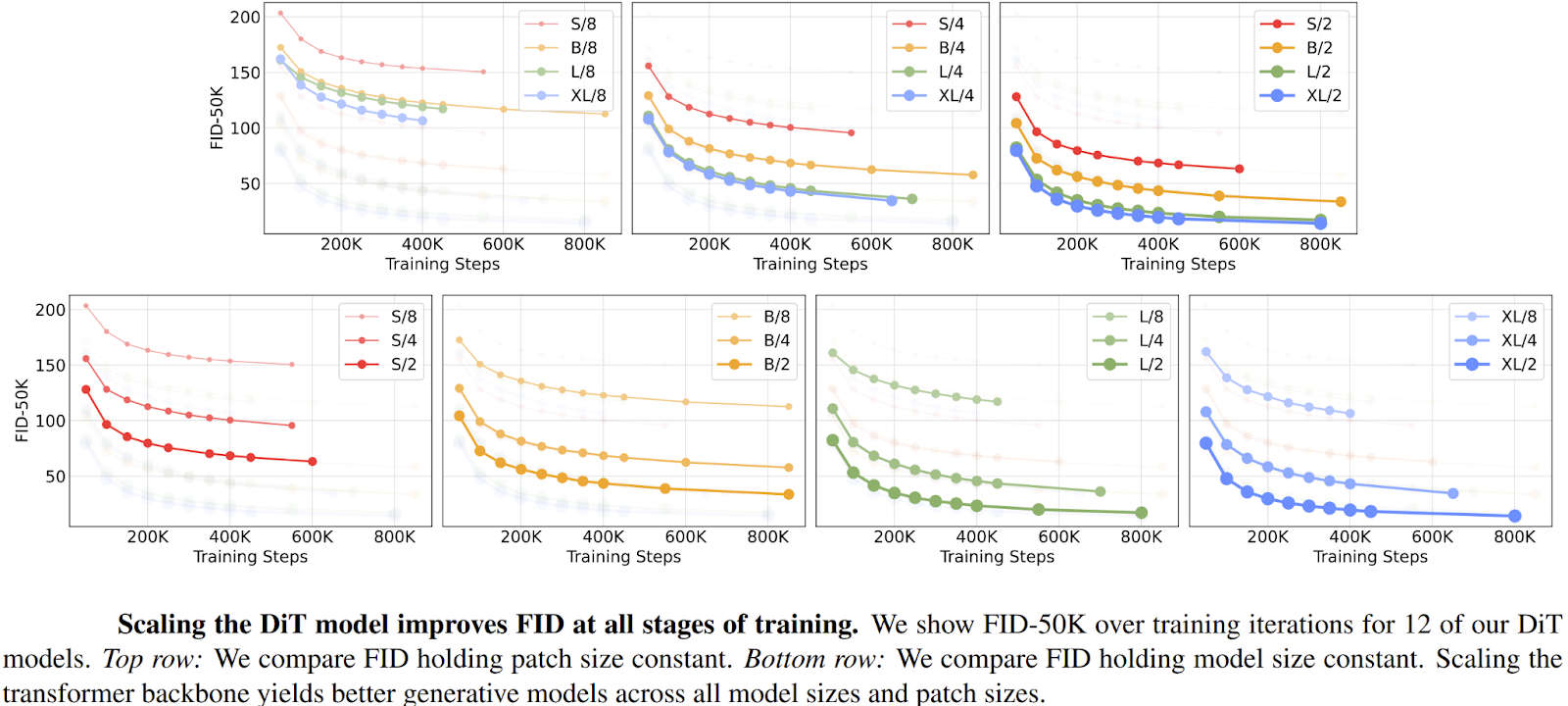
The key finding was a strong, predictable relationship: models with higher Gflops consistently achieved lower (better) FID scores. The Gflops of a DiT could be increased in three main ways:
- Increasing model depth (stacking more DiT blocks).
- Increasing model width (using larger hidden dimensions).
- Increasing the number of input tokens (using a smaller patch size, e.g., patch-size=2).
This direct correlation proved that, just like in other domains, investing more compute into a transformer-based diffusion model yields predictably better results.
This scaling hypothesis was put to the test with the largest model configuration, named DiT-XL/2. The "XL" denotes an extra-large model, and "/2" refers to its use of a tiny 2x2 patch size, which maximizes the number of input tokens.
The performance of DiT-XL/2 was groundbreaking:
- On the class-conditional ImageNet 256x256 benchmark, DiT-XL/2 achieved a state-of-the-art FID of 2.27, significantly outperforming all previous diffusion models, whose best score was 3.60.
- On the more challenging 512x512 benchmark, DiT-XL/2 again set a new record with an FID of 3.04, beating the prior best of 3.85.
💡Pro Tip: When training large diffusion models, our NVIDIA B200 vs H100 benchmarks help you understand how newer GPU architectures impact attention-heavy workloads and training throughput.
While DiT-XL/2 is a computationally intensive model, it is remarkably efficient compared to previous state-of-the-art models that operated in pixel space. By processing compact latent representations instead of full-resolution images, DiTs drastically reduce the computational burden.
For example, on the 256x256 benchmark, the DiT-XL/2 model requires approximately 119 Gflops per forward pass. In contrast, the previous top-performing pixel-space model (ADM-U) required 742 Gflops to achieve a lower-quality result. This efficiency becomes even more pronounced at higher resolutions, demonstrating the immense advantage of operating in a latent space.
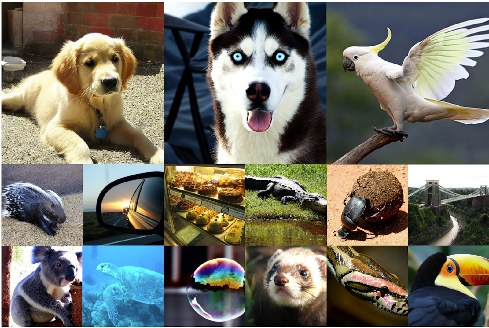
Ultimately, the strong performance and scaling properties of DiTs confirmed that a general-purpose, scalable architecture like the transformer could outperform specialized, convolutional designs like the U-Net, marking a pivotal moment in the evolution of generative models.
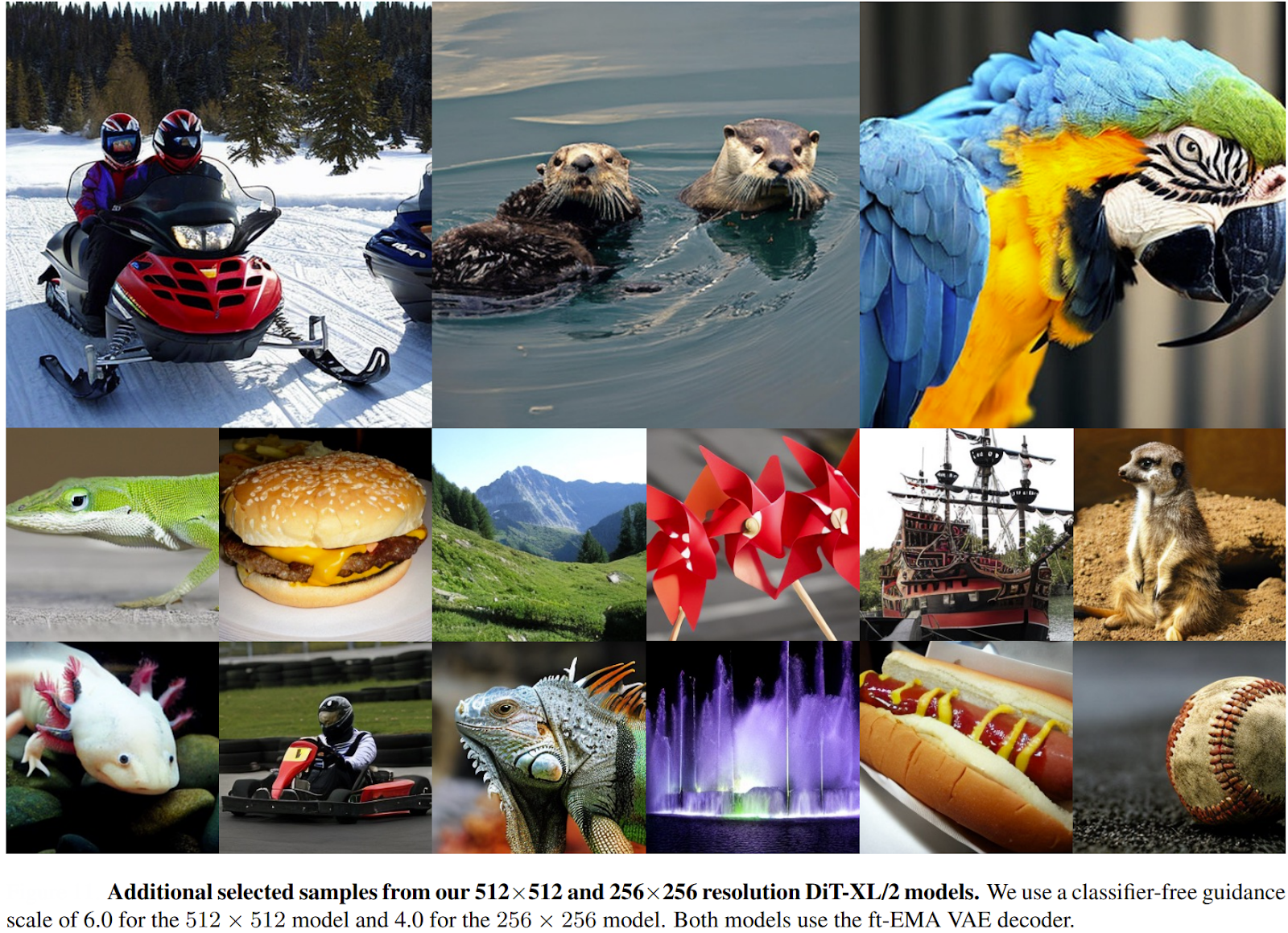
Some qualitative examples generated by DiTs are shown below.
Applications and State-of-the-Art Developments
The success of DiTs has made them a foundational architecture, inspiring a wave of innovation across various domains of generative AI. Researchers are now actively applying, adapting, and scaling DiT principles to tackle new challenges, from generating video to enhancing images and even designing molecules.
Here are a few key areas where DiTs are making a significant impact:
Video Generation
The ability of transformers to model sequences makes them a natural fit for video generation, which requires understanding both spatial details within a frame and temporal relationships across frames.
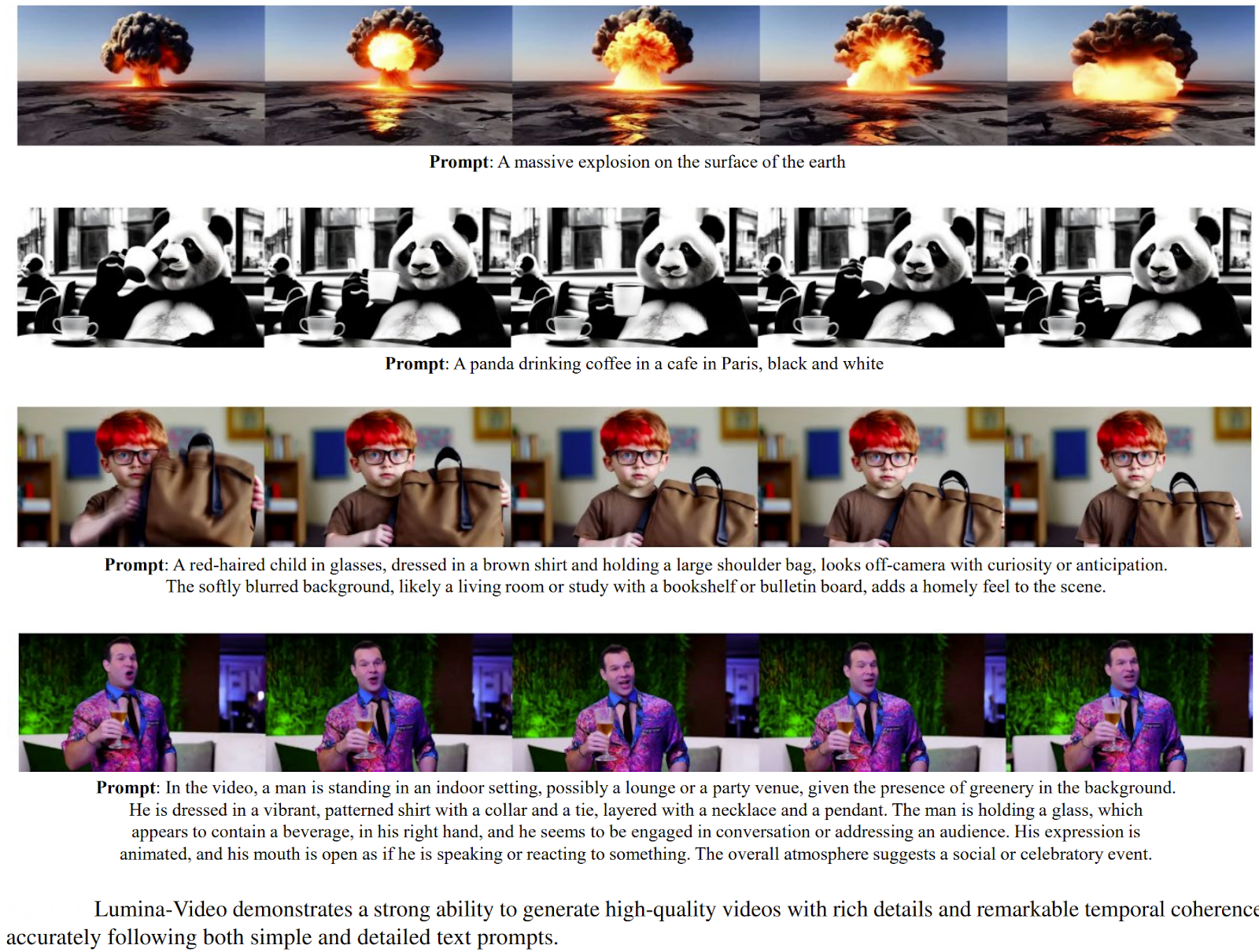
Models like Lumina-Video adapt the DiT framework to handle spatiotemporal data by jointly learning from multiple patch sizes. This multi-scale approach not only improves efficiency but also allows for flexible control over the motion and dynamics in the generated videos, pushing the boundaries of high-quality video synthesis.
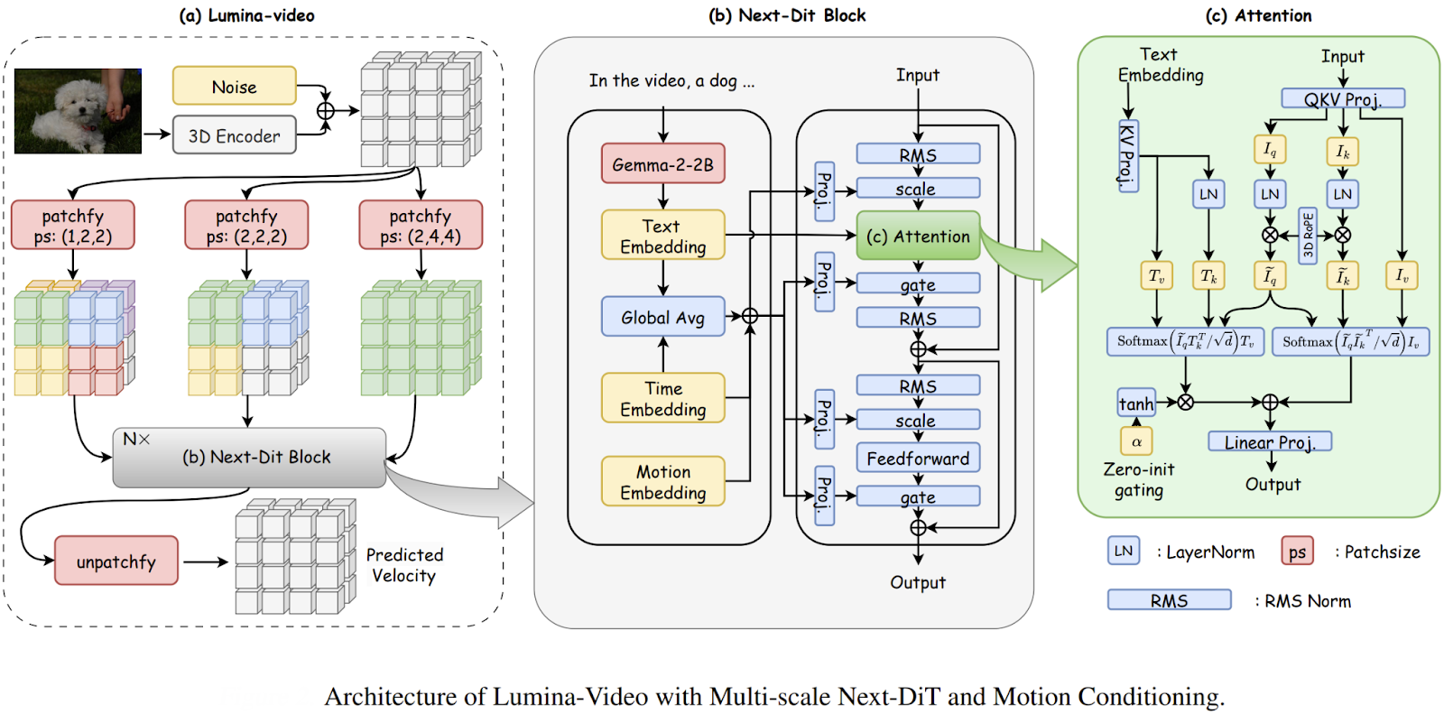
The core idea across many recent video models is to use DiT-based backbones with attention across both space and time to capture complex motion and maintain coherence.
Advanced Text-to-Image Generation
The original DiT paper focused on class-conditional generation, but the architecture has been rapidly adapted for more complex text-to-image tasks.
Recent work has focused on scaling these models to billions of parameters and training them on massive datasets with rich, descriptive captions.
💡Pro Tip: If you are interested in training models on languages with very little data, our Swiss-German LLMs article shows how to build strong language models in truly low-resource settings.
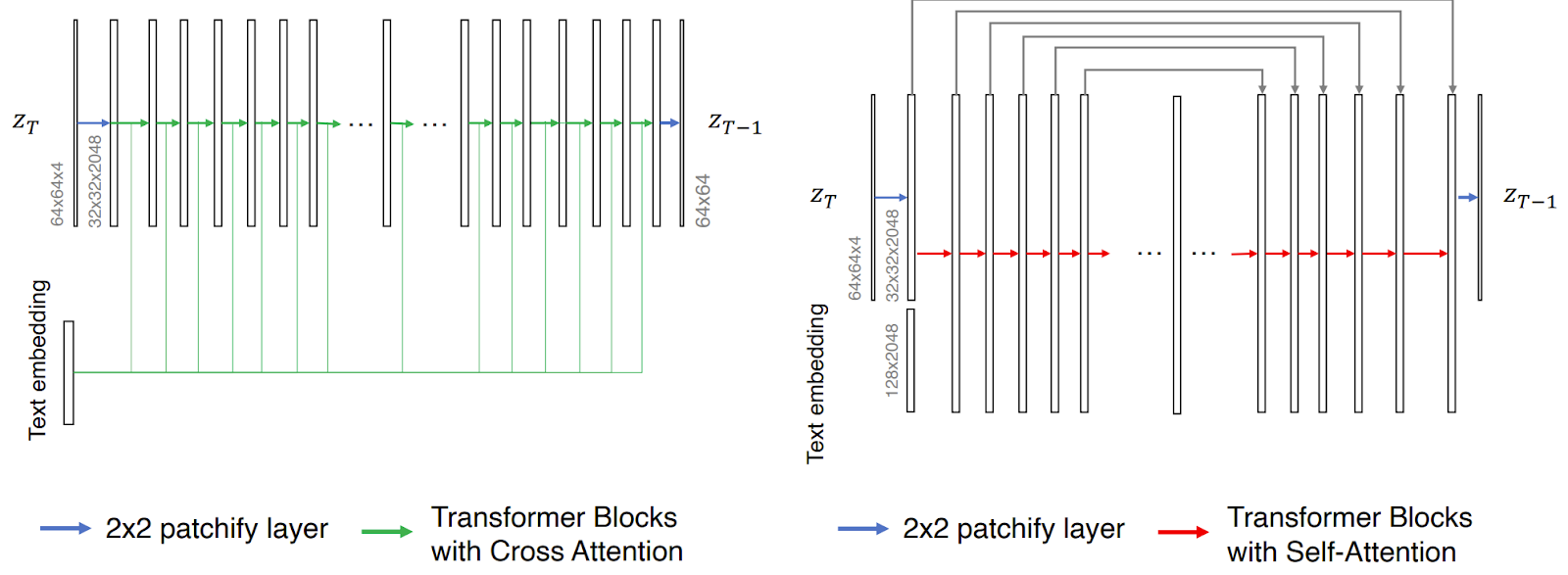
Research papers like "Efficient Scaling of Diffusion Transformers for Text-to-Image Generation" have rigorously studied different DiT variants, finding that simpler, pure self-attention designs (like U-ViT) can scale more effectively and even outperform more complex architectures in controlled settings.
This line of research is critical for building next-generation text-to-image models that offer greater prompt adherence and image quality.

Hybrid Architectures and Novel Paradigms
A significant development is the TransDiff model, which marries an Autoregressive (AR) Transformer with a diffusion model to create a unified generative framework.
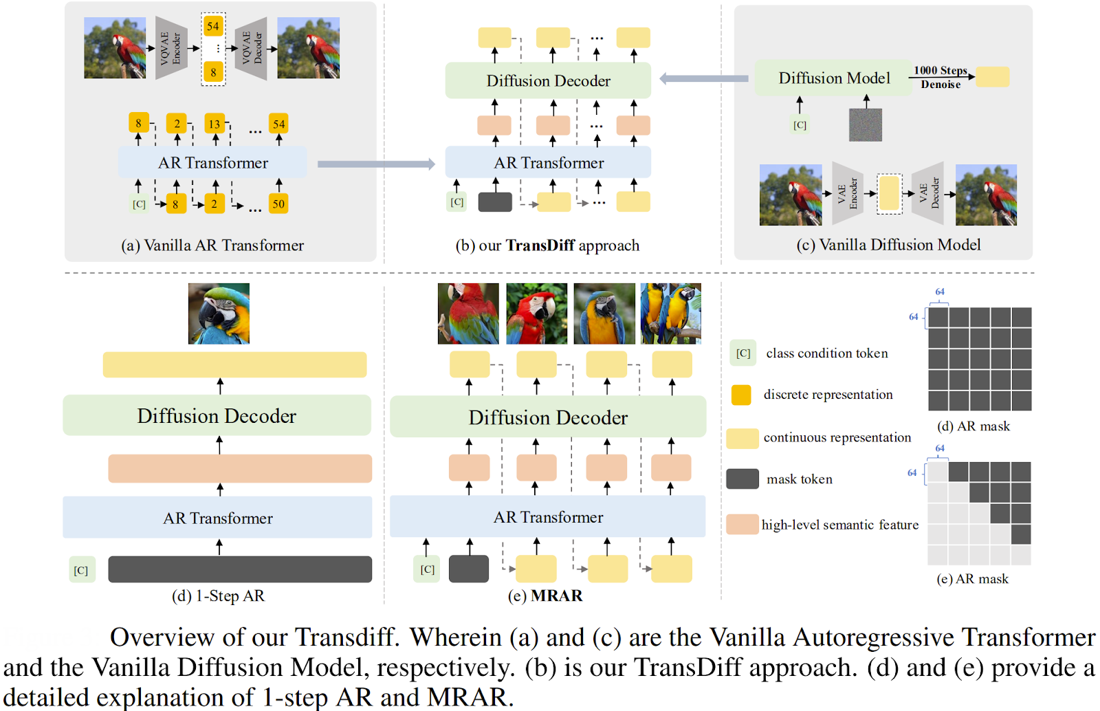
Instead of using a DiT for pure denoising, TransDiff employs an AR Transformer to encode an image into high-level semantic features. These features then act as a powerful conditioning signal for a diffusion decoder, which generates the final image.
This hybrid approach aims to combine the fast inference of AR models with the high quality of diffusion models, achieving state-of-the-art results on benchmarks like ImageNet with a reported FID score of 1.42. The work also introduces a novel training paradigm called Multi-Reference Autoregression (MRAR), which further improves generation quality and diversity.
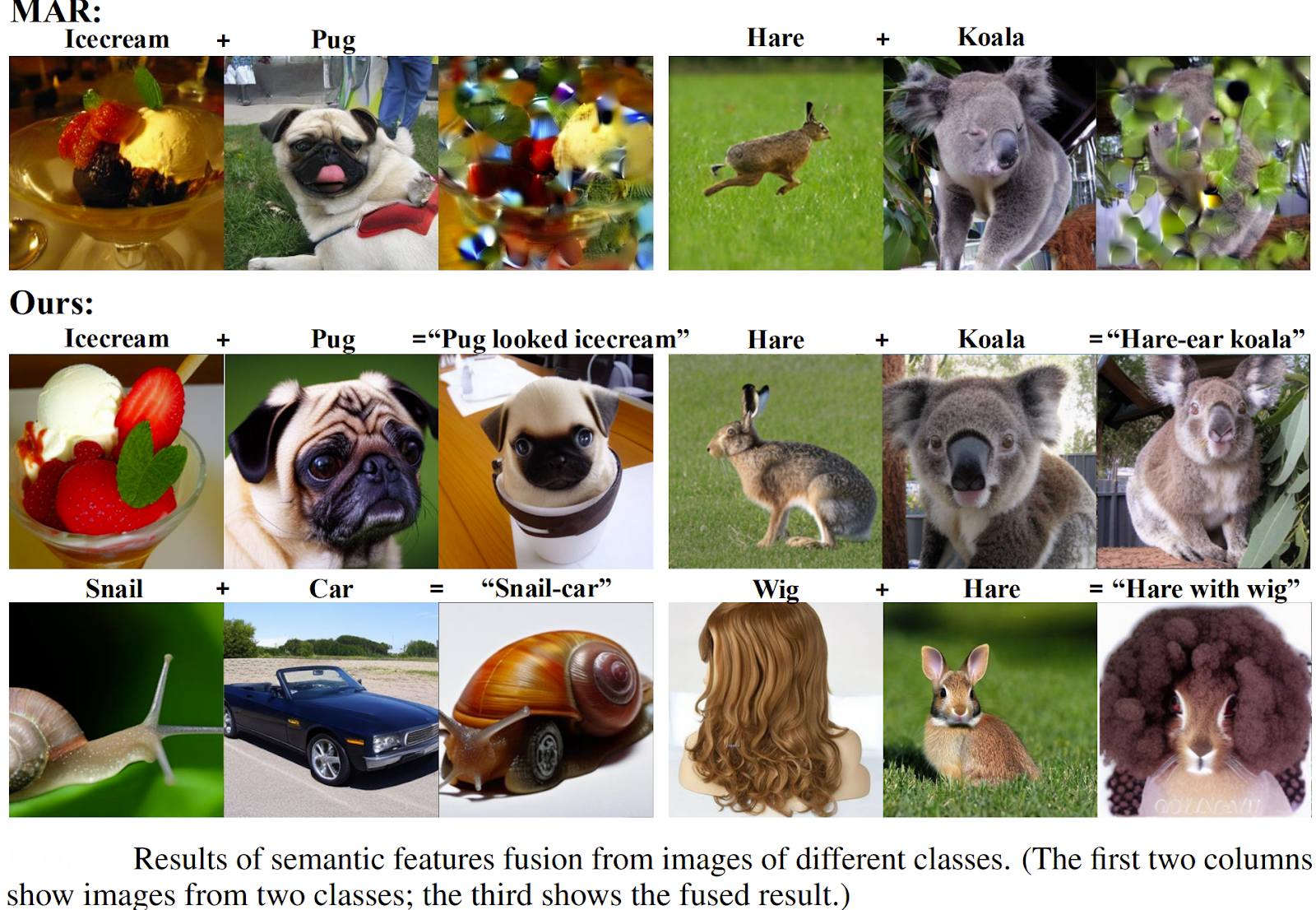
These examples represent just a fraction of the ongoing work. From scientific applications like molecular design to creative tools for artists and filmmakers, the DiT architecture is proving to be a robust and adaptable foundation for the future of generative modeling.
Diffusion Transformers: Key Takeaways
By replacing the long-standing U-Net architecture with a pure transformer backbone, DiTs have unlocked new levels of performance and scalability, fundamentally reshaping our understanding of what is required for state-of-the-art image synthesis.
As we've seen, it has already paved the way for groundbreaking applications in video generation, text-to-image synthesis, and even hybrid models that blend autoregressive and diffusion techniques for superior results.
Diffusion Transformers in a Nutshell:
- A New Architecture: Diffusion Transformers replace the traditional U-Net in diffusion models with a transformer, processing latent image patches as a sequence of tokens.
- Scalability is Key: DiTs demonstrate a clear and predictable scaling relationship—larger models with more computational power (Gflops) reliably produce higher-quality images (lower FID scores).
- Global Context Matters: By leveraging self-attention, DiTs can model long-range dependencies across an entire image at every step, a key advantage over locally-focused convolutional networks.
- State-of-the-Art Performance: The DiT-XL/2 model set new benchmarks for image generation, outperforming all previous diffusion models while being more computationally efficient by operating in a compressed latent space.
Foundation for the Future: The DiT architecture now serves as the backbone for many cutting-edge generative models, including OpenAI's Sora and Stability AI's Stable Diffusion 3, and continues to inspire new research into more efficient and powerful hybrid systems.

Stay ahead in computer vision
Get exclusive insights, tips, and updates from the Lightly.ai team.

.png)
.png)