Train Test Validation Split: Best Practices & Examples
Table of contents
Share blog post


The train-test-validation split is a best practice in machine learning to ensure models generalize well. Training data teaches the model, validation fine-tunes it, and the test set provides an unbiased evaluation on unseen data.
Share blog post
Understanding train test validation split is crucial for preventing overfitting and obtaining an unbiased assessment of model performance before deployment. Here’s a quick summary of key takeaways.
What is the train test validation split?
It is the process of dividing a dataset into three distinct subsets, which include training, validation, and test. Each subset serves a specific purpose in model development and evaluation.
- Training Set: The largest portion, used to train the machine learning model and optimize its internal model parameters.
- Validation Set: Used during the iterative process of model development to fine-tune the model's hyperparameters (like learning rate or regularization strength) and assess intermediate model performance to detect overfitting.
- Test Set: A completely held-out portion, used only once at the very end to provide an unbiased estimate of the final model accuracy on truly unseen data in real-world scenarios.
Why is train test validation split crucial for machine learning models?
It involves dividing a data set into three subsets - training, validation, and test - each serving a specific purpose in model development and evaluation.
What are the typical split ratios?
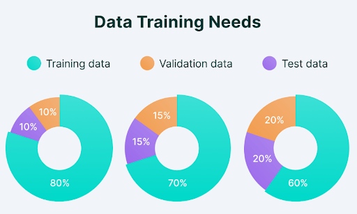
Common ratios include 70/15/15 and 80/10/10. For simpler train test splits, 80/20 is common.
What happens if a model does not split its data properly?
Overfitting - the model performs well on training data but poorly on new, unseen data - resulting in an unreliable assessment of model accuracy.
How does train test validation split relate to hyperparameter tuning and model evaluation?
The validation set tunes hyperparameters without touching the test set. The test set provides the final, unbiased model evaluation.
Train Test Validation Split: Best Practices & Examples
Building a machine learning model that performs well on training data is one thing. The true measure is how well it makes accurate predictions on completely unseen data in real-world scenarios.
This is where the train test validation split becomes a critical step in any ML project - the process of dividing data into distinct subsets, each playing a unique role in building and evaluating a trained model.
Here's what we will cover:
- Training, validation, and test sets: The core components
- Data splitting strategies: Best practices
- Implementing train test validation split in practice
- How to use Lightly for training, validation, and test splits
Getting the split right matters, but so does the quality of data in each set. At Lightly, we help you make smarter choices about what data to train, validate, and test on:
- LightlyStudio: Curate representative and diverse samples for each split, ensuring balanced coverage and fewer biases.
- LightlyTrain: Pretrain and fine-tune models on your domain-specific visual data - no labels needed for pretraining.
See Lightly in Action
Curate and label data, fine-tune foundation models — all in one platform.
Book a Demo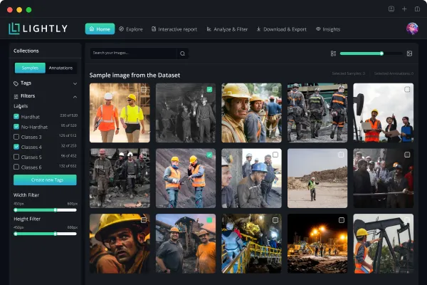
Building a machine learning model that performs well on training data is one thing. The true measure is how well it makes accurate predictions on completely unseen data in real-world scenarios.
This is where the train test validation split becomes a critical step in any ML project - the process of dividing data into distinct subsets, each playing a unique role in building and evaluating a trained model.
Here's what we will cover:
- Training, validation, and test sets: The core components
- Data splitting strategies: Best practices
- Implementing train test validation split in practice
- How to use Lightly for training, validation, and test splits
Getting the split right matters, but so does the quality of data in each set. At Lightly, we help you make smarter choices about what data to train, validate, and test on:
- LightlyStudio: Curate representative and diverse samples for each split, ensuring balanced coverage and fewer biases.
- LightlyTrain: Pretrain and fine-tune models on your domain-specific visual data - no labels needed for pretraining.
Training, Validation, and Test Sets: The Core Components
Before we dive into data splitting strategies and best practices, let's break down the role of each data set.
The Training Set
The training set contains most of the available data (typically 60-80% of the total data set) and is used to teach the machine learning model. It is the portion of the data set reserved to fit the model, allowing it to learn patterns and adjust its model parameters.
The model learns features and patterns in the training data. It improves its ability to link inputs to the right outputs by adjusting its internal model parameters based on prediction accuracy.
Key Characteristics of a Good Training Set
Your training set must be large enough and diverse to cover all scenarios. A training set that is too small or lacks diversity causes the model to either underfit or learn biased patterns that don't reflect real world data.
For example, if you want more diversity in your image training data with a balanced class distribution, you can do so with the LightlyStudio Selection feature. It allows you to specify a target class distribution and select images based on thresholding - for example, removing blurry images and keeping the sharpest ones.
Below is example code to select samples based on class distribution. See the complete guide for more selection use cases.
import os
import pickle
import numpy as np
from PIL import Image


# Helper to load a batch file
def load_batch(file):
    with open(file, 'rb') as f:
        return pickle.load(f, encoding='bytes')


# Create output directories
os.makedirs('cifar_images', exist_ok=True)


# Process training batches
for batch_id in range(1, 6):
    batch = load_batch(f'D:\lightly\cifar-10-batches-py\data_batch_{batch_id}')
    data = batch[b'data']      # shape (10000, 3072)
    for i in range(len(data)):
        img = data[i].reshape(3, 32, 32).transpose(1, 2, 0)
        img = Image.fromarray(img)
        img.save(f'cifar_images/img_{batch_id}_{i}.png')
The Validation Set
The validation set is a separate piece of the data set used to evaluate model performance during training. Unlike the training data, the model doesn't learn directly from the validation data. Instead, it helps assess how well the trained model handles new, unseen data.
The validation process also helps fine-tune hyperparameters and model configuration to improve overall model performance.
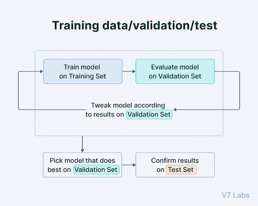
The Hyperparameter Tuning Cycle
When training a neural network or any other machine learning model, hyperparameter tuning follows a repetitive, iterative process:
- The model is initially trained on the training set.
- Model performance is evaluated on the validation set, either periodically or at the end of each epoch.
- Adjustments are made to hyperparameters like learning rate and regularization based on validation results. Changes can also be made to the model design, such as modifying layers or activation functions.
- Steps 1 to 3 are repeated until the model achieves adequate model performance on the validation set.
Key Consideration: If you tune the model too heavily to the validation data, you risk overfitting to it - reducing the model's ability to generalize to truly unseen data.
Note: "validation set" and "test set" are sometimes swapped in research papers. In this guide, validation = the set used during development for hyperparameter tuning; test = the held-out set evaluated only after training is complete.
The Test Set
The test set is an entirely separate part of the data (typically 10-20% of the total data set), kept aside from both training and validation data. It evaluates final model performance after training is complete.
The test set provides an unbiased evaluation of how well the trained model generalizes to unseen data, and assesses its capabilities in real-world scenarios.
Protecting the Test Set from Contamination
The test set should be isolated before any data preprocessing, scaling, or feature engineering - to avoid data leakage. Never use test data to make model development decisions. Even evaluating test results to decide whether to keep training is a form of "peeking" that compromises final model performance measurement.
Also ensure zero duplicate examples across the training set, validation set, and test set. Duplicates allow the model to memorize records rather than learn generalizable patterns, inflating model accuracy.
The table below summarizes each data set's role, purpose, and timing in the machine learning workflow.
Why Three Sets Are Often Better Than Two
Using two groups - training and testing - is common. But dividing data into three parts is generally better for machine learning model evaluation.
The primary reason for having a separate validation set is to avoid using the test set repeatedly to tune the model. Doing so causes the test set to lose its ability to give an unbiased estimate of final model performance on new data.
For large data sets, a ratio like 98/1/1 can be used to maximize training data while still allowing for validation and testing - even 1% of a million-record data set is statistically significant. For most projects, common split ratios are 60/20/20, 80/10/10, and 70/15/15.
Pro tip: Splitting your data the right way is only half the battle - choosing the right tools matters too. Check out our list of the Top Computer Vision Tools in 2026 to find the best fit for your next project.
Common Data Splitting Strategies: Best Practices
When preparing data sets for machine learning, there is no single best approach. The right data splitting strategy depends on the type of data you have (images, time series, grouped samples, etc.) and the challenges you want to avoid (bias, imbalance, or leakage).
Below are the most common data splitting strategies, along with when to use them.
Random Splitting
Random sampling mixes up all the data and splits it into training, validation, and test groups based on predetermined percentages.
Random splitting helps prevent biases that might otherwise consistently affect a single subset. It is best for large, varied data sets where each data point is independent and evenly represented. Random sampling is not the correct approach for imbalanced data sets or data with group structure.
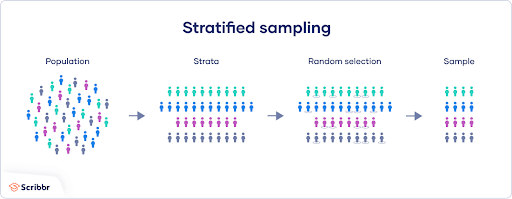
Stratified Splitting
Stratified sampling divides a data set while keeping the original class distribution in each subset.
Stratified splitting is the correct approach for imbalanced data sets, where some classes have very few samples. A random split might accidentally concentrate all rare-class examples in the test set. Stratified sampling ensures the same class distribution appears in the training set, validation set, and test set, producing class balanced data sets across all splits.
For example, if your data set has 90% cats and 10% dogs, stratified splitting ensures that same proportion is maintained in your training data, validation data, and test data.
Time-Based Splitting
When working with time series data - such as stock prices, weather patterns, or sensor readings - standard random sampling is inappropriate. Instead, split the data based on time: use earlier data for training and later data for testing.
Time-based splitting reflects real-life scenarios where models predict future events using only past data, preventing data leakage from future observations into training data.
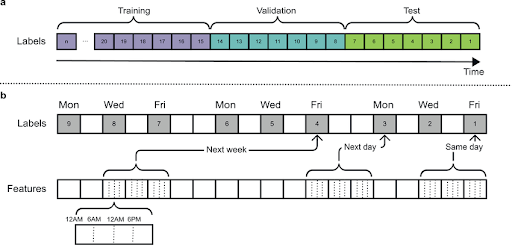
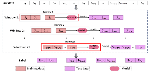
Advanced methods like rolling window validation or walk-forward validation move the training period forward in time step by step, testing the model on the next period each time.
Group Splitting
Group splitting is for data sets where data points belong to logical groups - for example, multiple scans from the same patient, or frames from the same video.
It ensures all data points from a single group stay together in either the training set, validation set, or test set. Without it, data from the same patient or video could appear in both training and validation data, producing an unfairly optimistic model performance estimate.
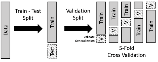
Cross Validation Splitting
Cross validation creates multiple data subsets, each used as a training set or validation set in different cross validation iterations. It provides more reliable machine learning model performance metrics than a single train test split, especially for smaller data sets where a fixed split may not be statistically representative.
K Fold Cross Validation in Practice
K fold cross validation divides the data set into k equal-sized folds. The machine learning model trains on k-1 folds and is evaluated on the remaining fold, repeating until each fold has served as the validation set. Results are averaged into a reliable model performance estimate not dependent on a single train test split.
Stratified K Fold Cross Validation
Stratified k fold cross validation ensures each fold maintains the same class distribution as the original data set - essential for imbalanced data sets and fair model evaluation across all classes.
Domain-Aware Splitting
Standard splits assume test data and training data come from the same distribution (i.i.d.), which often isn't true in practice. Real-world applications encounter domain shift, where deployment data differs from training data.
Adversarial validation uses a discriminator model to detect domain shift between training and validation sets. Domain-free adversarial splitting (DFAS) creates train validation test splits by maximizing domain differences between subsets, training the model to generalize across that boundary.
Clustering-Based Splitting for Small Data Sets
For small data sets (typically under a few thousand samples), standard random or stratified approaches can produce splits with poor distributional coverage. Clustering-based splitting groups similar samples using K-Means or HDBSCAN first, then draws samples proportionally from each cluster for each split.
This maintains the distributional structure of the data set better than random sampling alone - useful in domains like medical imaging or industrial inspection where labeled training data is scarce.
The table below gives a quick comparison of the most common data splitting methods.
Implementing Train Test Validation Split in Practice
Besides selecting the right data splitting method, following best practices is crucial to keep your data reliable and your machine learning model trustworthy.
How to Implement Train Test Validation Split with scikit-learn
scikit-learn's train_test_split is the standard tool for data splitting in Python. It supports shuffling, stratification, and a configurable test size for both two-way and three-way splits.
Basic Train Test Split
from sklearn.model_selection import train_test_split

# 80/20 train test split
X_train, X_test, y_train, y_test = train_test_split(
    X,
    y,
    test_size=0.2,
    random_state=42
)
Three-Way Train Test Validation Split
To produce a three-way split (70/15/15), apply train_test_split twice - first to split off the test set, then to divide the remaining training and validation data:
from sklearn.model_selection import train_test_split

# Step 1: hold out 15% as the test set
X_train_val, X_test, y_train_val, y_test = train_test_split(
    X,
    y,
    test_size=0.15,
    random_state=42
)

# Step 2: from the remaining 85%, hold out ~17.6% as validation
# (0.176 * 0.85 ≈ 0.15 of the full data set)
X_train, X_val, y_train, y_val = train_test_split(
    X_train_val,
    y_train_val,
    test_size=0.176,
    random_state=42
)
For imbalanced data sets, add stratify=y to preserve class distribution across the training set and test set:
from sklearn.model_selection import train_test_split

X_train, X_test, y_train, y_test = train_test_split(
    X,
    y,
    test_size=0.2,
    stratify=y,
    random_state=42
)
NumPy can also be used for custom data splitting logic via manual indexing. For cross validation purposes, scikit-learn's KFold and StratifiedKFold classes provide k fold cross validation directly.
Preventing Data Leakage: The Silent Killer of Model Performance
Data leakage occurs when information from the validation set or test set leaks into the training data, producing overly optimistic model performance metrics and inflated final model accuracy.
Types of Data Leakage
- Target leakage: A feature contains information about the target variable that wouldn't be available at prediction time - for example, using a downstream outcome as a feature when predicting that same target variable.
- Feature leakage: A feature indirectly encodes the target variable through a correlated proxy.
- Temporal leakage: Future data contaminates training data in time series problems.
- Preprocessing leakage: Normalization or scaling is fit on the full data set rather than only the training set.
For specialized domains like bioinformatics and computational chemistry, DataSAIL (Nature Communications, April 2025) provides leakage-reduced splitting for out-of-distribution evaluation scenarios.
Strategies to Overcome Data Leakage
To prevent data from leaking between training and testing, apply these strategies:
- Isolate Test Set Early: Set aside the test set before any data preprocessing, feature engineering, or data augmentation.
- Apply Transformations Consistently: Fit scaling or normalization only on the training set, then apply the same parameters to validation data and test data without recalculating.
- Time-Aware Splitting: For time series, split chronologically so that future data doesn't affect training.
- Group-Aware Splitting: For correlated data - such as by patient ID or video sequence - keep whole groups together in one split.
Data Augmentation and Data Splitting Order
Data augmentation increases the size and diversity of the training data by applying transformations like rotating, flipping, cropping, or color changes to images.
The correct approach is to split training and validation data first, then apply augmentation only to the training set. Applying augmentation before splitting can cause identical images to appear in both training and validation data, producing overly optimistic model accuracy estimates. Augmenting validation data also reduces its value, since real-world data isn't typically augmented.
Mistakes You Need to Avoid When Data Splitting
- Poor Training Set Quality: If your training set is too small, not diverse enough, or low quality, the machine learning model won't learn the right patterns. Inadequate sample size leads to unreliable model performance metrics.
- Improper Shuffling: Shuffle your data before splitting. Improper shuffling introduces bias, causing the model to exploit patterns not representative of unseen data.
- Over-tuning to the Validation Set: Repeatedly adjusting the model based on validation results can cause overfitting to the validation data, undermining model evaluation integrity.
- Duplicate Examples: Ensure zero duplicate examples across training, validation, and test sets. Duplicates inflate model accuracy and final model performance estimates.
How to use Lightly for Training, Validation, and Test Splits
When starting a computer vision project, there is an immense amount of raw training data to handle, and labeling all of it is expensive. Using random sampling may result in redundant images or missing rare scenes that undermine model performance.
The Lightly platform helps you pick the best data and create splits with minimal manual effort. It uses embedding-based strategies like DIVERSITY and TYPICALITY to ensure training and validation data is diverse, representative, and of high quality. With LightlyStudio, you can scale active learning: select the most valuable subsets for training, validation, and testing from raw image data.
1. Install the Lightly Python client package
pip install lightly2. Download the LightlyStudio Worker
docker pull lightly/worker:latest

docker run --shm-size="1024m" --rm lightly/worker:latest sanity_check=True
While the worker is being downloaded, you can continue with step 3.
3. Prepare Image Data
We'll download and use the CIFAR-10 data set here. Alternatively, you can use your own data set or the sample clothing data set from Lightly.
curl -L -o cifar-10-python.tar.gz https://www.cs.toronto.edu/~kriz/cifar-10-python.tar.gzUnzip the image data to a folder:
tar -xzf cifar-10-python.tar.gzThen, convert batches to PNG images:
import os
import pickle
import numpy as np
from PIL import Image


def load_batch(file):
    with open(file, "rb") as f:
        return pickle.load(f, encoding="bytes")


os.makedirs("cifar_images", exist_ok=True)

for batch_id in range(1, 6):
    batch = load_batch(f"cifar-10-batches-py/data_batch_{batch_id}")
    data = batch[b"data"]

    for i in range(len(data)):
        img = data[i].reshape(3, 32, 32).transpose(1, 2, 0)
        img = Image.fromarray(img)
        img.save(f"cifar_images/img_{batch_id}_{i}.png")
4. Schedule a Selection run
Get your LightlyStudio token from app.lightly.ai/preferences. Set it as LIGHTLY_TOKEN in your environment or code.
from os import linesep
from pathlib import Path
from datetime import datetime

import platform
import torch

from lightly.api import ApiWorkflowClient
from lightly.openapi_generated.swagger_client import DatasetType, DatasourcePurpose


# Change these two variables
LIGHTLY_TOKEN = "CHANGE_ME_TO_YOUR_TOKEN"  # Copy from https://app.lightly.ai/preferences
DATASET_PATH = Path("/path/to/cifar_images")


assert DATASET_PATH.exists(), f"Dataset path {DATASET_PATH} does not exist."

client = ApiWorkflowClient(token=LIGHTLY_TOKEN)

client.create_dataset(
    dataset_name=f"first_dataset__{datetime.now().strftime('%Y_%m_%d__%H_%M_%S')}",
    dataset_type=DatasetType.IMAGES,
)

client.set_local_config(purpose=DatasourcePurpose.INPUT)
client.set_local_config(purpose=DatasourcePurpose.LIGHTLY)

scheduled_run_id = client.schedule_compute_worker_run(
    worker_config={
        "shutdown_when_job_finished": True
    },
    selection_config={
        "n_samples": 500,
        "proportion_samples": 0.1,
        "strategies": [
            {
                "input": {
                    "type": "EMBEDDINGS"
                },
                "strategy": {
                    "type": "DIVERSITY"
                }
            },
            {
                "input": {
                    "type": "METADATA",
                    "key": "lightly.sharpness"
                },
                "strategy": {
                    "type": "THRESHOLD",
                    "threshold": 20,
                    "operation": "BIGGER"
                }
            }
        ]
    },
)

gpus_flag = "--gpus all" if torch.cuda.is_available() else ""
omp_num_threads_flag = " -e OMP_NUM_THREADS=1" if platform.system() == "Darwin" else ""

print(
    f"{linesep}Docker Run command:{linesep}"
    f"docker run{gpus_flag}{omp_num_threads_flag} --shm-size='1024m' --rm -it \\{linesep}"
    f"\t-v '{DATASET_PATH.absolute()}':/input_mount:ro \\{linesep}"
    f"\t-v '{Path('lightly').absolute()}':/lightly_mount \\{linesep}"
    f"\t-e LIGHTLY_TOKEN={LIGHTLY_TOKEN} \\{linesep}"
    f"\tlightly/worker:latest{linesep}"
)

print(
    f"{linesep}Lightly Serve command:{linesep}"
    f"lightly-serve \\{linesep}"
    f"\tinput_mount='{DATASET_PATH.absolute()}' \\{linesep}"
    f"\tlightly_mount='{Path('lightly').absolute()}'{linesep}"
)
5. Process the run with the LightlyStudio Worker
Run the Docker command, and the worker will take a while to process your data set.
docker run --shm-size=1024m --rm \
  -v /path/to/cifar_images:/input_mount:ro \
  -v /path/to/lightly:/lightly_mount \
  -e LIGHTLY_TOKEN=YOUR_TOKEN \
  lightly/worker:latest
6. Explore the selected training set
View and explore the selected training data interactively on the LightlyStudio platform using the Lightly serve command.
lightly-serve \
  input_mount="/path/to/cifar_images" \
  lightly_mount="/path/to/lightly"
Download the text file (.txt) containing the selected training image filenames. The code below copies the chosen training images from your raw image folder to a separate folder.
import os
import shutil


selected_train = []

with open("selected_filenames.txt") as f:
    for line in f:
        fname = line.strip().split(",")[0]
        selected_train.append(fname)

os.makedirs("cifar10_split/train", exist_ok=True)

for fname in selected_train:
    src = os.path.join("cifar_images", fname)
    dst = os.path.join("cifar10_split/train", fname)

    if os.path.exists(src):
        shutil.copy(src, dst)
        print(f"Copied: {fname}")
    else:
        print(f"File not found: {src}")
Use DIVERSITY and THRESHOLD strategies to maximize visual coverage and reduce redundancy in the training set. Set n_samples to 70-80% of your data.
Repeat the same approach for validation and test sets with different strategies:
- Validation set: TYPICALITY to reflect the overall data set distribution (10-15% of data).
- Test set: DIVERSITY to cover edge cases and challenging examples (10-15% of data).
Exclude already-chosen images from each new selection to prevent duplicate examples across splits.
Using LightlyTrain on the Training Set
With the training set in hand, we can pretrain a model using LightlyTrain. LightlyTrain is a self-supervised pretraining and fine-tuning framework for domain-specific visual data. As of April 2026 (version 0.15.0), it supports YOLO (v5-v12), RT-DETR, RF-DETR, DINOv2, DINOv3, ResNet, and other architectures from Torchvision, TIMM, and Ultralytics. No labeled training data is needed for pretraining.
1. Install the LightlyTrain package
pip install lightly2. Pretrain the model
import lightly_train

dataset_path = "./cifar10_split/train"

if __name__ == "__main__":
    lightly_train.train(
        out="out/my_experiment",
        data=dataset_path,
        model="torchvision/resnet50",
        epochs=2,
        batch_size=32,
    )
Once training is complete, the output directory contains:
out/my_experiment/
├── checkpoints/
│   ├── epoch=99-step=123.ckpt
│   └── last.ckpt
├── events.out.tfevents.123.0
├── exported_models/
│   └── exported_last.pt
├── metrics.jsonl
└── train.log
The final model is exported to out/my_experiment/exported_models/exported_last.pt and can be used directly for fine-tuning on classification tasks, detection, or segmentation.
Frequently Asked Questions
What is the train test split for validation?
A train test split divides a data set into two subsets: one for training and one for testing. When you add a separate validation set, the two-way train test split becomes a three-way train test validation split.
In a train test validation split, the validation set sits between the training set and the test set in the workflow. The training set teaches the model; the validation set tunes hyperparameters and monitors model performance during training; and the test set is held out entirely, evaluated only once at the end to give an unbiased measure of how well the trained model generalizes to unseen data.
The key distinction: training and validation data influence model development decisions, while test data does not.
What is a good train test valid split?
A good train test valid split depends on the size of your data set. Common ratios are:
- 70/15/15: Provides more data for validation and testing; useful when careful model evaluation is a priority.
- 80/10/10: Maximizes training data while keeping enough for validation and testing; the most common choice.
- 60/20/20: More data for model evaluation; useful for smaller data sets or complex classification tasks.
For large data sets with millions of records, a 98/1/1 split can still provide statistically significant validation and test sets. For small data sets, k fold cross validation is often better than a fixed train validation test split, since it uses all the data for both training and validation across folds and produces more reliable evaluation metrics.
Neural networks typically need more training data than simpler models, which pushes the ratio toward 80/10/10 or higher.
Why 80/20 train test split?
The 80/20 train test split is widely used because it balances maximizing training data with retaining enough test data for reliable model performance evaluation.
It reflects a general principle that more training data leads to better model performance - particularly for neural networks, which require large amounts of training data to learn complex patterns.
scikit-learn's train_test_split defaults to a 75/25 split, and 80/20 is a common override. The optimal ratio depends on data set size, model complexity, and specific model evaluation requirements. For very large data sets, you can often reduce the test split below 20% while still achieving statistically significant evaluation metrics.
Is a train test split needed for cross validation?
Yes - a separate test split is still needed even when using cross validation. Cross validation uses multiple train test validation splits within the training data to produce a more reliable model performance estimate than a single validation split. However, it does not replace the held-out test set.
The correct approach: first split off a test set that is never touched during cross validation, then apply k fold cross validation within the remaining training and validation data. Each fold creates a temporary train test split, but final model performance is always reported on the separate test set.
Reporting only cross validation results can produce optimistic estimates, since model selection decisions are influenced by the cross validation results on the same data set.
Key Takeaways: Mastering Data Splitting
The train test validation split brings reliability to building machine learning models. The way you split your training data, validation data, and test data directly affects how well your model learns and generalizes in the real world.
From simple random splits to advanced strategies for time series, imbalanced classes, or domain shift, the best data splitting approach depends on your data and goals. With the right strategy, you can create training, validation, and test sets that accurately measure model performance and prepare your trained model for truly unseen data.

Stay ahead in computer vision
Get exclusive insights, tips, and updates from the Lightly.ai team.


.png)
.png)