‍

Deep neural networks can take weeks to train from scratch on large datasets and require substantial computing power.

Luckily, this time can be shortened using transfer learning. 

It lets you reuse pre-trained model weights for new, related tasks in computer vision and natural language processing (NLP).

In this guide, we will cover:

1. What is Transfer Learning?
2. How Does Transfer Learning Work?
3. Types and Strategies of Transfer Learning
4. Applications of Transfer Learning
5. Advantages and Challenges of Transfer Learning
6. How Can Lightly AI Help With Your Transfer Learning Requirements?

Transfer learning pipelines depend on quality data, the effective use of unlabeled information, and efficient training methods. 

At Lightly, we ensure data quality and help you get the most out of unlabeled data through:

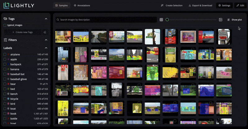
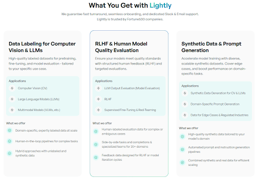
• LightlyStudio helps curate, clean, analyze (data preparation), and annotate your vision and text data. It uses embedding-based selection to focus effort on the most informative samples that improve the relevance of data.

• LightlyTrain addresses pretraining and feature learning. It uses self-supervised algorithms to pretrain models on unlabeled domain images. The result is a foundation (base) model that needs less labeled data for fine-tuning.

• When you don’t have enough labels or need to cover edge cases, then request our AI Data Services. We provide expert-led annotated datasets (for computer vision, LLMs, and custom AI development) to improve models for few-shot or specialized applications.

Interested in training your own vision foundation model? Check out LightlyTrain!

What is Transfer Learning? 

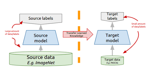
Transfer learning (TL) is a machine learning technique where a model trained on one task (source task) is reused as the starting point for a different, but related task (target task).

This method uses the knowledge gained (the learned weights or features) from the initial task to speed up the learning process on new data.

To put it simply, we are repurposing an existing model for a new job.

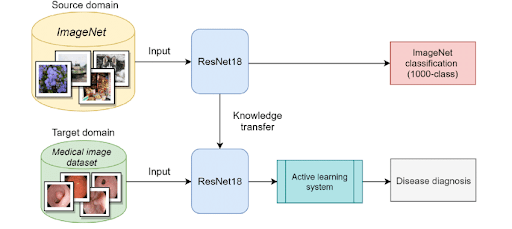
For example, a convolutional neural network (CNN) trained on millions of ImageNet images has already learned to detect edges, textures, and general pixel-level patterns. 

We can take that ImageNet-trained model and fine-tune (adapt) it to recognize agricultural images or specific objects (new task). 

We often need fewer examples of the new labeled data to reach good accuracy by starting with a pretrained model’s weights (since TL yielded faster convergence).

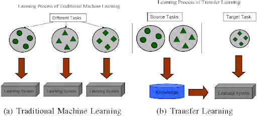
Now, let's compare the two types of learning (transfer learning vs. training from scratch).

‍

Let’s now take a look at how transfer learning works.

How Does Transfer Learning Work? (Process and Steps)

Transferring knowledge to a machine-learning model for a new task involves several key steps.

Select a Pre-Trained Model (Initial Training) 

The first step is to get the pre-trained model with prior knowledge or skills for a related task. And you have two main options: either use a public model or pre-train your own for custom domains.

For many common tasks, you can use a public pre-trained model and weights from a library like TensorFlow Hub, PyTorch, or HuggingFace.

For computer vision, this is typically a CNN like ResNet or EfficientNet that was pretrained on a large dataset. For NLP, this might be a foundation model like BERT.

In case your target domain is very unique, like satellite imagery, medical scans, or manufacturing defects, a generic ImageNet model may struggle. Then, the best strategy is to pre-train a model's weights on your own data.

To do this, you can use LightlyTrain. It automates state-of-the-art SSL (self-supervised learning) on your unlabeled image data to create a pretrained model that understands the features and data distribution of your domain.

This custom initial training leads to much higher model performance when you later fine-tune on your limited data.

LightlyTrain supports a wide range of vision backbones. It includes Torchvision CNNs (ResNet, ConvNeXt, ShuffleNet), TIMM models (ViTs, ConvNets), Ultralytics YOLO (v5 to v12), DETR variants (RT-DETR, RF-DETR), and more.

Here is the script for pretraining Torchvision models (resnet18) with LightlyTrain as an example:

import lightly_train


if __name__ == "__main__":
    lightly_train.train(
        out="out/my_experiment",                # Output directory.
        data="my_data_dir",                     # Directory with images.
        model="torchvision/resnet18",           # Pass the Torchvision model.
    )

Or alternatively, pass a Torchvision model instance directly:

from torchvision.models import resnet18


import lightly_train


if __name__ == "__main__":
    model = resnet18()                        # Load the Torchvision model.
    lightly_train.train(
        out="out/my_experiment",              # Output directory.
        data="my_data_dir",                   # Directory with images.
        model=model,                          # Pass the Torchvision model.
    )

Freeze and Reuse Early “Generic” Layers

In the pretrained network, the early layers usually learn general features (detecting simple pixel values or basic shapes).

In many TL scenarios, we freeze these layers so their settings (weights) do not change during training.

These frozen layers act as a fixed feature extractor and provide the knowledge they learned from the initial task.

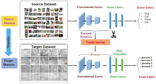
Replace or Add New Layers (Task-Specific Adaptation) 

The later layers of the original model were specialized for its source task’s outputs (classifying 1,000 ImageNet objects). 

We remove these layers and add new, untrained layers that match the target task.

For example, if your new goal is image classification for 10 types of products, you add a new head with 5 outputs. These new layers will learn the task-specific features you need.

Fine-Tune on Target Data

Finally, we train (or fine-tune) the model on the target data.

We typically train the newly added layers from scratch (as they started randomly) and also unfreeze some of the later pretrained layers if the target dataset is large enough. 

To continue after pretraining with LightlyTrain, export the weights from out/my_experiment/exported_models/exported_last.pt and load them into your preferred ML framework for fine-tuning. Otherwise, you can use weights that you have already downloaded.

Below is a simple example using PyTorch:

import torch
import torchvision.transforms.v2 as v2
import tqdm
from torch import nn, optim
from torch.utils.data import DataLoader
from torchvision import datasets, models


transform = v2.Compose([
    v2.Resize((224, 224)),
    v2.ToImage(),
    v2.ToDtype(torch.float32, scale=True),
])
dataset = datasets.ImageFolder(root="my_data_dir", transform=transform)
dataloader = DataLoader(dataset, batch_size=16, shuffle=True, drop_last=True)


# Load the exported model
model = models.resnet18()
model.load_state_dict(torch.load("out/my_experiment/exported_models/exported_last.pt", weights_only=True))


# Update the classification head with the correct number of classes
model.fc = nn.Linear(model.fc.in_features, len(dataset.classes))


device = "cuda" if torch.cuda.is_available() else "mps" if torch.backends.mps.is_available() else "cpu"
model.to(device)


criterion = nn.CrossEntropyLoss()
optimizer = optim.Adam(model.parameters(), lr=0.001)
print("Starting fine-tuning...")
num_epochs = 10
for epoch in range(num_epochs):
    running_loss = 0.0
    progress_bar = tqdm.tqdm(dataloader, desc=f"Epoch {epoch+1}/{num_epochs}")
    for inputs, labels in progress_bar:
        optimizer.zero_grad()
        outputs = model(inputs.to(device))
        loss = criterion(outputs, labels.to(device))
        loss.backward()
        optimizer.step()
        progress_bar.set_postfix(loss=f"{loss.item():.4f}")
    print(f"Epoch [{epoch+1}/{num_epochs}], Loss: {loss.item():.4f}")

Throughout this process, we evaluate the model on a validation set to monitor model performance. If needed, adjust hyperparameters or try unfreezing more layers gradually. 

The goal is to balance reusing generic knowledge with learning enough new information so the model makes accurate predictions on the target domain. 

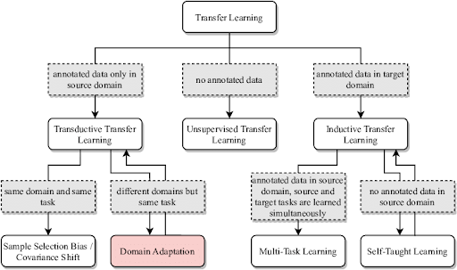
Types of Transfer Learning (Inductive vs. Transductive vs. Unsupervised)

Transfer learning methods are grouped into three types based on the task and data available: inductive, transductive, and unsupervised transfer learning.

Inductive transfer learning uses labeled target data where source and target domains are the same, but the tasks the model is working on differ. 

On the other hand, transductive transfer learning refers to the case where the task remains the same but the domains shift, and we don’t have labels for the target data.

Pro tip: If you are looking for a data labeling tool, check out this list of 12 Best Data Annotation Tools for Computer Vision (Free & Paid).

In unsupervised transfer learning, there are no labels in either the source or target data. Models learn general patterns from one dataset and use that knowledge to work with another dataset.

Here is a side-by-side comparison of these three types:

‍

Transfer Learning Strategies: Fine-Tuning, Frozen Layers, and Feature Extraction

There are two strategies to transfer the pretrained model knowledge to the target task: feature extraction and fine-tuning.

In feature extraction, we freeze all or most of the pretrained model’s layers and use them as a fixed feature extractor for the new task. Only train the new layers (classifier or regressor) on the target data.

The feature extraction strategy is the go-to choice when your target dataset is small or similar to the original. It's fast to train and has a lower risk of overfitting limited data.

In contrast, fine-tuning unfreezes some layers (or all) of the pre-trained model and trains them (along with the new layers) on the target data.

Fine-tuning works well when you have a reasonable amount of labeled data for your new task. It often gives better accuracy than pure feature extraction, but costs more computation and risks overfitting if the target data is limited.

Pro tip: Check out 5 Best Data Annotation Companies in 2025 [Services & Pricing Comparison].

Modern ML data pipelines use both approaches (hybrid). First, train only the new layers (with base frozen) to get the new head initialized. Then fine-tune some of the base layers with a smaller learning rate.

Applications of Transfer Learning

Transfer learning is standard practice for building high-performance models for real-world applications in computer vision and NLP.

Computer Vision

Computer vision models need to learn to recognize features from pixel values. A model trained on a large image dataset has already learned to identify edges, textures, and shapes. And that knowledge is extremely valuable for new tasks, including.

Image Classification: Pretrained CNNs serve as backbones for new classification tasks. For example, a ResNet or VGG model pretrained on millions of images can be fine-tuned on a smaller dataset (wildlife or medical images). And it yields much higher accuracy than training a CNN from scratch.

‍Object Detection and Segmentation: Detection frameworks (Faster R-CNN, YOLO) and segmentation models (U-Net) often use pretrained networks as feature extractors (to find features in an image). A pretrained model provides strong feature representations that speed up training of detectors and improve final performance.

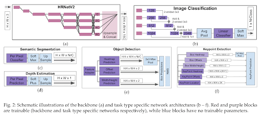
Style Transfer and Domain Adaptation: Models trained on one style or domain (synthetic images) can be adapted to another (real photos) using TL techniques. 

For example, this paper uses HRNet-based approaches, where high-resolution features enable smoother adaptation across domains. Features preserve spatial details and improve performance in dense prediction tasks such as segmentation, detection, and keypoint estimation.

Natural Language Processing (NLP)

NLP models had to learn language from scratch for every task before transfer learning. Now, large foundation models are pre-trained on a massive amount of text from the internet and can help perform many language tasks.

• Text Classification (Sentiment Analysis): A model like BERT is pretrained to understand the rules and context of language. You can fine-tune it on a small dataset of labeled reviews to perform sentiment analysis. As the model already has language understanding, it only needs to learn how to map that understanding to your specific labels (positive or negative). 

• Other NLP Tasks: This same idea applies to many other tasks. Pretrained models like BERT and GPT are fine-tuned to perform question answering, text summarization, and named entity recognition (NER).

Other Domains and Use Cases

Besides its uses in computer vision (CV) and natural language processing (NLP), transfer learning is also used in many other fields. 

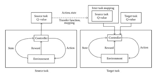
For example, in reinforcement learning (RL), an agent (such as a robot) can be trained in a safe simulation (the source task). The knowledge gained (its policy) can then be transferred to a real-world robot (the target task). 

Likewise, a clean English speech audio model can be fine-tuned for use in noisy environments or for different dialects (a new data distribution). 

In healthcare and biotech, models trained on medical data or chemical compounds can transfer knowledge to related tasks, such as new disease diagnosis or molecular property prediction.

Advantages of Transfer Learning

Transfer learning provides considerable benefits compared to training a model from scratch, including.

• Reduced Data Requirements: Deep neural networks normally need massive amounts of labeled data. Since transfer learning models start with general knowledge, they don’t require as many examples of the new task to learn.
  
  
• Shorter Training Time and Lower Compute Cost: A pretrained model needs only a few epochs of fine-tuning to converge on the new task (as you start with a highly capable existing model). It greatly reduces training time and computing resources compared to training a large model from scratch.
  
  
• Better Generalization (Avoiding Overfitting): A model trained from scratch on limited data is likely to overfit (memorize the training examples). Because a pretrained model starts with general knowledge, it is less likely to overfit your small dataset and can improve performance on the real-world target domain.

• Lower Need for From-Scratch Model Development: You don’t need to develop or train a deep network from zero. You can take an existing neural network architecture and weights (such as a ResNet or BERT) and adapt them to save design and training effort.

Challenges and Limitations of Transfer Learning

Despite its advantages, transfer learning has potential pitfalls:

• Negative Transfer: If the source and target tasks (or domains) are too different, transferring knowledge can hurt performance instead of helping (using a model trained on medical X-rays to identify street signs).

• Solution: Select a source model that was pre-trained on a task or domain as similar as possible to your target. If no similar model, then pretrain your own domain-specific model with LightyTrain. See the sample code below for pretraining a YOLOv12 model:

import lightly_train


if __name__ == "__main__":
    lightly_train.train(
        out="out/my_experiment",                # Output directory.
        data="my_data_dir",                     # Directory with images.
        model="ultralytics/yolov12s.yaml",      # Pass the YOLO model.
    )


# Or alternatively, pass directly a YOLOv12 model instance:


from ultralytics import YOLO


import lightly_train


if __name__ == "__main__":
    model = YOLO("yolov12s.yaml")               # Load the YOLOv12 model.
    lightly_train.train(
        out="out/my_experiment",                # Output directory.
        data="my_data_dir",                     # Directory with images.
        model=model,                            # Pass the YOLOv12 model.
    )

• Data Distribution Shift: Even if the task is the same, a shift in data distribution between source and target (domain shift) can degrade performance. For example, a model trained on clear, well-lit photos (one data distribution) may perform poorly on a target domain of blurry, nighttime photos (a different distribution).

• Solution: Use data augmentation to make your training data look more like the target data. Or use a data-centric platform like LightlyStudio to select target data that bridges this gap. Studio offers a feature to perform automated data selection to pick samples that are both representative (typical) and diverse (novel).

from lightly_studio.selection.selection_config import (
    MetadataWeightingStrategy,
    EmbeddingDiversityStrategy,
)
...
# Compute typicality and store it as `typicality` metadata
dataset.compute_typicality_metadata(metadata_name="typicality")


# Select 10 samples by combining typicality and diversity, diversity
dataset.query().selection().multi_strategies(
    n_samples_to_select=10,
    selection_result_tag_name="multi_strategy_selection",
    selection_strategies=[
        MetadataWeightingStrategy(metadata_key="typicality", strength=1.0),
        EmbeddingDiversityStrategy(embedding_model_name="my_model_name", strength=2.0),
    ],
)

• Model Size and Cost: Many pre-trained foundation models, such as GPT-3 and vision transformers, are huge. Fine-tuning or even loading them requires a lot of memory and GPU/TPU resources. 

• Solution: Consider knowledge distillation to transfer the expertise of a large teacher model like DINOv2 ViT-B/14 into your smaller architecture like resnet18. Fine-tuning smaller model variants (DistilBERT instead of BERT for the NLP case) or using parameter-efficient fine-tuning (PEFT) methods. Follow the code below to pretrain and distill your own weights (DINOv2 for now) in LightlyTrain.

import lightly_train


if __name__ == "__main__":
    # Pretrain a DINOv2 ViT-B/14 model.
    lightly_train.train(
        out="out/my_dinov2_pretrain_experiment",
        data="my_dinov2_pretrain_data_dir",
        model="dinov2/vitb14",
        method="dinov2",
    )


    # Distill the pretrained DINOv2 model to a ResNet-18 student model.
    lightly_train.train(
        out="out/my_distillation_pretrain_experiment",
        data="my_distillation_pretrain_data_dir",
        model="torchvision/resnet18",
        method="distillation",
        method_args={
            "teacher": "dinov2/vitb14",
            "teacher_weights": "out/my_dinov2_pretrain_experiment/exported_models/exported_last.pt", # pretrained `dinov2/vitb14` weights
        }
    )

• Overfitting in Fine-Tuning: If the target dataset is small, fine-tuning can still overfit to that limited data, especially when too many layers are unfrozen.

• Solution: Use aggressive data augmentation and regularization, or keep more layers frozen and only train the final head of the model.

How Can Lightly AI Help With Your Transfer Learning Requirements?

Lightly AI offers a computer vision suite that enables you to pretrain models, including foundation models, for multiple computer vision tasks.

LightlyStudio helps build the best possible image dataset for fine-tuning. It makes data curation and labeling easier by identifying the most informative samples so that the training data is diverse and aligned with the target domain. 

This curated dataset can then be used for transfer learning to produce accurate models, with lower labeling and training costs than those involved in training the original model.

LightlyTrain supports customizing and improving models for various vision tasks using self-supervised learning. 

It also enables you to scale down large models to make them more efficient for real-world use through knowledge distillation.

Furthermore, Lightly AI Data Services offers expert data labeling and creates synthetic data to expand small datasets, which is a major challenge in transfer learning.

Conclusion

Transfer learning is a jump-start for new machine learning tasks. It enables handling complex image and language tasks with limited data and resources.

We can make our models perform better on new data by using knowledge from previous tasks. To do this, we choose a pretrained model and either keep some parts the same (freeze) or adjust them (fine-tune).

With tools and services such as LightlyStudio, LightlyTrain, and AI Data Service, transfer learning workflows become even more efficient.