‍

Introduction

Training a machine learning model is never perfect on the first run. Models adjust, struggle, and slowly improve, but only when they are pointed in the right direction. 

In PyTorch, the selection of loss functions is a key part of the learning path, alongside the optimizer, learning rate, data, and regularization.

In this article, we will discuss the most popular PyTorch loss functions, how they are used in various tasks, and how to apply them in practice.

Here’s what we will cover:

1. What is a loss function in PyTorch?
2. Types of loss functions in PyTorch
3. Regression loss functions in PyTorch
4. Classification loss functions in PyTorch
5. Ranking and metric learning loss functions
6. Combining Multiple Loss Functions (Multi-Task Learning)
7. Implementing Custom Loss Functions in PyTorch
8. Loss Functions in Semi-Supervised and Active Learning (Advanced Applications)

Choosing the right loss function is important, but the quality and selection of your training data play an equally critical role in model performance. 

At Lightly, we help you get the most out of your PyTorch workflows with:

• LightlyTrain: Pretrain and fine-tune models for better convergence and improved performance across different tasks.
  
• LightlyOne: Curate the most diverse and informative samples to make each training step more efficient and impactful.

Together, they complement your loss function strategy and help you train models that generalize better with less effort.

What Is a Loss Function in PyTorch? 

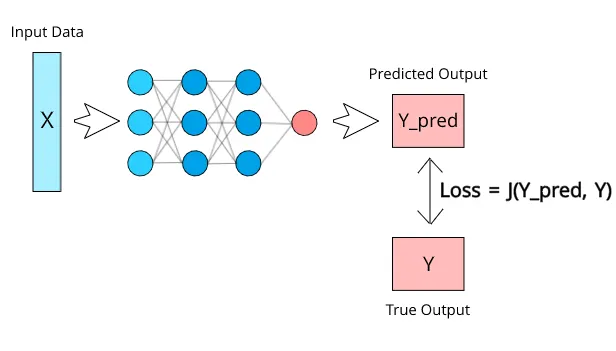
A loss function is a mathematical formula that takes the model’s predicted output and the target values (the ground truth), then calculates a single number, the loss value. This number represents the “error” or “distance” between the model's prediction and the actual value.

Different tasks call for various kinds of loss functions. The decision is based on whether you are working with continuous values or discrete categories. 

All the standard loss functions in PyTorch are available in the torch.nn module (usually imported as import torch.nn as nn). To use them, you just call the loss function with the model’s predictions and the target values. 

PyTorch takes care of the rest and gives you a single loss value you can use for optimization.

Many loss functions first calculate the error for each sample or output, then reduce those values into a single number. By default, PyTorch uses 'mean' reduction, so you get the average loss across the batch.

This behavior can be changed using the reduction argument:

• reduction='mean': average of all losses (default)
• reduction='sum': total sum of all losses
• reduction='none': returns per-sample losses without reducing

This gives you flexibility in how the loss is computed and used during training.

Types of Loss Functions in PyTorch 

PyTorch offers a range of loss functions designed for different kinds of learning tasks, mainly regression, classification, and ranking.

For regression tasks, loss functions focus on the distance between actual and predicted values. The error is measured as either a mean squared error, mean absolute error, or smooth L1, depending on whether sensitivity to outliers matters.

Classification losses compare logits with labels, relying on activation functions like softmax or sigmoid.

Meanwhile, ranking and similarity-based losses don’t just look at single predictions. They judge the relative distances between multiple outputs, teaching models to order or group them meaningfully.

Comparison of Common PyTorch Loss Functions

The table below compares the most common PyTorch loss functions and the scenarios they are best suited for.

‍

Proper selection emphasizes loss value, guiding the optimization algorithms to improve model performance.

Regression Loss Functions in PyTorch

Regression tasks predict continuous values (prices, pixel intensities). The goal is to minimize the gap between the actual and predicted values on a numeric scale.

In practice, you select between absolute difference and squared error based on how you want to handle outliers and significant mistakes.

PyTorch provides regression losses through torch.nn (as criterion classes) and torch.nn.functional (as functional forms). These are used as loss functions applied to predicted and target tensors. 

Let’s look at some types of regression loss functions:

Mean Absolute Error (L1 Loss)

L1 Loss computes the average absolute difference between predicted and actual values. It handles outliers better than squared error and provides stable gradients. This makes it well-suited for training on noisy data.

In PyTorch, you can use it as nn.L1Loss. It minimizes elementwise errors by default using the 'mean', but you can change the reduction parameter to 'sum' or 'none' to gain more control.

Let’s review the PyTorch implementation code.

loss_fn = nn.L1Loss()  # default reduction='mean'
 
# Example predicted and actual values
pred = torch.tensor([2.5, 0.0, 2.1]) 	# predicted values
target = torch.tensor([3.0, -1.0, 2.0])  # target values (ground truth)
 
# Compute loss value
loss_val = loss_fn(pred, target)
print(loss_val.item())  # mean absolute error

Use floating-point tensors and keep prediction/target shapes consistent to ensure stable gradient computation and reliable training behavior. Modify the reduction method to 'none' if per-sample errors are required.

Pro tip: If you’re working on object detection tasks, understanding evaluation metrics is just as important as picking the right loss function. Check out our guide to Mean Average Precision (mAP) to learn how to measure detection performance effectively.

Mean Squared Error (L2 Loss)

L2 Loss (or Mean Squared Error Loss) computes the average squared difference between predicted and actual values. Penalizing squared differences emphasizes large deviations, encouraging the model to reduce bigger errors in regression.

In PyTorch, you can use nn.MSELoss to compute the mean squared error loss.

loss_fn = nn.MSELoss()  # default reduction='mean'
pred   = torch.tensor([2.5, 0.0, 2.1], dtype=torch.float32)  # predicted values
target = torch.tensor([3.0, -1.0, 2.0], dtype=torch.float32) # target values
 
loss_val = loss_fn(pred, target)
print(loss_val.item())  # mean squared error

Maintain consistent float tensors, set requires_grad=True on model parameters for backprop updates, and choose a matching reduction for training to ensure proper learning signals.

Smooth L1 Loss (Huber Loss)

Smooth L1 Loss, also referred to as Huber Loss, is a combination of L1 and L2 loss. On small errors, it acts like squared error with smooth gradients, but on large errors (transition threshold), it becomes linear, limiting the influence of outliers. 

In object detection, it is commonly used for bounding box regression, where it balances precision with robustness to noisy annotations.

In PyTorch, you can implement it as nn.SmoothL1Loss(beta=1.0, reduction='mean'). Adjust the beta and reduction according to the requirements.

loss_fn = nn.SmoothL1Loss()  # behaves like MSE for small errors, L1 for large
pred   = torch.tensor([2.5, 0.0, 2.1], dtype=torch.float32)
target = torch.tensor([3.0, -1.0, 2.0], dtype=torch.float32)
loss_val = loss_fn(pred, target)
print(loss_val.item()) 

You can use this in tasks that need precise error measurement but must avoid being dominated by outliers (e.g., bounding box regression).

Classification Loss Functions in PyTorch

In classification tasks, the model outputs continuous logits rather than discrete categories. Classification losses compare these logits (or their implied probabilities) to the true labels. 

Instead of comparing raw numbers, these losses work with probability distributions generated by activation functions such as the sigmoid function or softmax function.

Binary Cross-Entropy

Binary Cross-Entropy (BCE) compares the probability distribution of predictions and the target values in binary classification problems. The model produces raw logits, and BCEWithLogitsLoss applies sigmoid activation internally to ensure stability.

It is commonly applied to multi-label classification, where each label is independent of the other.

In PyTorch, nn.BCEWithLogitsLoss is used, which combines sigmoid activation with BCE.

loss_fn = nn.BCEWithLogitsLoss()
 
# Example for binary classification
pred   = torch.tensor([0.8, -1.2, 2.0], dtype=torch.float32)   # raw logits
target = torch.tensor([1.0, 0.0, 1.0], dtype=torch.float32)	# target values
 
loss_val = loss_fn(pred, target)
print(loss_val.item())

Cross-Entropy Loss 

Cross-entropy Loss is used for multi-class, single-label classification, where each input belongs to exactly one class. 

It penalizes the difference between the true class label (as a probability distribution) and the predicted distribution, computed internally using softmax on the logits.

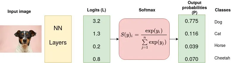
In PyTorch, nn.CrossEntropyLoss expects logits of shape (N, C) and integer class targets of shape (N,) with dtype torch.long.

loss_fn = nn.CrossEntropyLoss()
 
# Example for multi-class classification
pred   = torch.tensor([[2.0, 0.5, 1.0],   # logits for sample 1
                   	[0.1, 1.2, 2.1]],  # logits for sample 2
                  	dtype=torch.float32)
 
target = torch.tensor([0, 2])  # true class indices
 
loss_val = loss_fn(pred, target)
print(loss_val.item())

Negative Log Likelihood Loss 

NLLLoss expects the model output to be log-probabilities, unlike CrossEntropyLoss, which applies softmax internally. It penalizes the model when the correct class has a low log-probability.

Pairing it with a log_softmax layer is equivalent to computing the cross-entropy loss. 

Here is the simple implementation for NLLLoss in PyTorch:

loss_fn = nn.NLLLoss()
 
# Example: applying log_softmax before passing to NLLLoss
pred = torch.tensor([[2.0, 0.5, 1.0],
                 	[0.1, 1.2, 2.1]], dtype=torch.float32)
 
log_probs = F.log_softmax(pred, dim=1)
target = torch.tensor([0, 2])  # true class indices
 
loss_val = loss_fn(log_probs, target)
print(loss_val.item())

With nn.NLLLoss, it is important to note that the input tensor should contain log-probabilities and not logits or probabilities.

In PyTorch, apply CrossEntropyLoss to multi-class, single-label classification and BCEWithLogitsLoss to binary or multi-label classification. The two functions receive raw logits as input, as they internally apply softmax or sigmoid to ensure numerical stability.

Other Classification Losses & Considerations

In PyTorch, when using loss functions, it is crucial to know how they process activations, inputs, reductions, and generalization, which directly impact training stability and performance.

Here are some of the points you might consider:

Activation Handling: Some losses, like nn.CrossEntropyLoss (softmax) and nn.BCEWithLogitsLoss (sigmoid), apply activations internally, while others, like nn.NLLLoss, require manual activation (log-softmax).

Overconfidence & Smoothing: Overconfident predictions can hurt generalization. Label smoothing mitigates this by softening targets and improving robustness.

Numerical Stability: Use stable variants when available (e.g., nn.BCEWithLogitsLoss instead of sigmoid + BCE) to avoid issues like vanishing gradients or null values.

The table below summarizes some other classification losses:

‍

Ranking and Metric Learning Loss Functions

Unlike standard classification loss functions or regression tasks, these losses focus on the relationships between input tensors rather than their exact match with target values.

They are used in deep learning for information retrieval and semi-supervised tasks, where the structure of the embedding space is more important than predicting specific values.

Pro tip: Many ranking and metric learning methods benefit from strong feature representations learned through self-supervised learning. Check out our guide to Self-Supervised Learning (SSL) to understand how these techniques improve embedding quality and downstream performance.

Hinge Embedding Loss (Similarity-Based)

HingeEmbeddingLoss is designed for tasks where input pairs are labeled as either similar (+1) or dissimilar (-1). It promotes embeddings of similar inputs to come closer together, while separating those that are unlike.

The loss value depends on the absolute difference (distance) between embeddings and a margin hyperparameter.

This loss is effective in binary classification tasks framed as similarity problems. A common case is in Siamese networks, where two input images can be compared for image classification.

hinge_loss = nn.HingeEmbeddingLoss(margin=2.0)
 
# Suppose we have embeddings for two inputs
emb_a = torch.tensor([1.0, 2.0], requires_grad=True)
emb_b = torch.tensor([1.5, 2.5], requires_grad=True)
 
# Compute distance (Euclidean here)
dist = F.pairwise_distance(emb_a.unsqueeze(0), emb_b.unsqueeze(0), p=2)
 
# Label: +1 means similar, -1 means dissimilar
sim_label = torch.tensor([1])
 
loss_val = hinge_loss(dist, sim_label)
print(loss_val.item())

• When sim_label = +1, the loss function will minimize the distance between embeddings (bringing them closer).
• If sim_label = -1, the loss ensures they are at least a certain margin apart.

This balance helps the model build an embedding space where two probability distributions (similar vs. dissimilar) are clearly separated.

Cosine Embedding Loss

The CosineEmbeddingLoss compares similarity based on the cosine angle between two vectors. Rather than using raw magnitude, it evaluates how aligned their directions are.

A label of +1 pushes the embeddings closer by increasing their cosine similarity. A label of -1 pushes them apart, ensuring they are separated by at least the defined margin.

This makes it suitable for tasks like semantic similarity, document matching, and cross-modal embedding learning.

In PyTorch, you can use nn.CosineEmbeddingLoss(margin).

cos_loss = nn.CosineEmbeddingLoss(margin=0.5)  # margin ∈ [-1, 1]
emb_a = torch.tensor([[0.8, 0.6]], dtype=torch.float32, requires_grad=True)
emb_b = torch.tensor([[0.7, 0.7]], dtype=torch.float32, requires_grad=True)
sim_label = torch.tensor([1])  # +1 similar, -1 dissimilar
 
loss_val = cos_loss(emb_a, emb_b, sim_label)

Margin Ranking Loss

The MarginRankingLoss enforces a relative order on two predictions to ensure one score is ranked higher than the other by a margin.

Rather than aiming for absolute correctness, ranking loss functions represent preferences and are used in ranking systems like search engines and recommender models.

In PyTorch, use nn.MarginRankingLoss(margin) with a small positive margin (e.g., 1.0) to avoid trivial ties.

rank_loss = nn.MarginRankingLoss(margin=1.0)
output1 = torch.tensor([2.3], dtype=torch.float32, requires_grad=True)  # score for item A
output2 = torch.tensor([1.1], dtype=torch.float32, requires_grad=True)  # score for item B
target  = torch.tensor([1.0])  # y=1 → output1 should rank above output2
 
loss_val = rank_loss(output1, output2, target)

Triplet Margin Loss

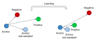
The TripletMarginLoss generalizes ranking to triplets, an anchor, a positive (same class as the anchor), and a negative (different class). The goal is to pull the anchor closer to positive and push it further away from negative by at least a given margin.

This is important in metric learning tasks where the model must learn embeddings that generalize well to unseen classes, such as in face recognition or verification.

In PyTorch, use nn.TripletMarginLoss(margin, p). p=2 applies Euclidean distance, while p=1 uses Manhattan distance.

triplet_loss = nn.TripletMarginLoss(margin=1.0, p=2) 
anchor   = torch.tensor([[0.5, 0.7]], dtype=torch.float32, requires_grad=True)
positive = torch.tensor([[0.52, 0.72]], dtype=torch.float32, requires_grad=True)
negative = torch.tensor([[1.5, -0.3]], dtype=torch.float32, requires_grad=True)
 
loss_val = triplet_loss(anchor, positive, negative)

Kullback–Leibler Divergence Loss (KLDivLoss)

KLDivLoss measures divergence between two probability distributions. It is frequently applied in knowledge distillation, variational autoencoders (VAEs), and semi-supervised learning, where point labels are less relevant than distributions. 

In PyTorch, the nn.KLDivLoss expects the input to be log-probabilities (F.log_softmax) and the target to be probabilities (F.softmax). This asymmetry is consistent with the KL formula and numerically stable.

student_logits = torch.tensor([[2.0, 0.5, -1.0]])
teacher_logits = torch.tensor([[1.5, 0.7, 0.3]])
 
student_log_probs = F.log_softmax(student_logits, dim=1)  # input: log-probs
teacher_probs = F.softmax(teacher_logits, dim=1)      	# target: probs
 
loss_fn = nn.KLDivLoss(reduction="batchmean")
loss_val = loss_fn(student_log_probs, teacher_probs)

Combining Multiple Loss Functions (Multi-Task Learning)

Neural networks often need to handle more than one goal at a time, like classifying inputs, predicting continuous values, and learning useful embeddings. This may require combining different loss functions and getting an overall measure.

In PyTorch, since loss values are tensors, you can easily combine them by taking a weighted sum. The gradients will automatically adjust to train a task-specific network during backpropagation.

Weighted Combination of Losses

The loss scales may differ widely when different objectives are combined. For example, CrossEntropyLoss values are typically in a low range (often below ~5), while regression losses like SmoothL1Loss can be smaller in scale depending on the data.

This imbalance of losses may lead to one loss becoming dominant in the training signal, causing inefficient learning dynamics. You can either do manual weighting (w_cls, w_reg, etc.) or dynamic reweighting to solve this issue.

# Example: weighted combination
total_loss = w_cls * cls_loss + w_reg * reg_loss
total_loss.backward()  # gradients propagate through both losses

If tasks differ significantly in scale, gradients may still be unbalanced even with advanced weighting methods like GradNorm or uncertainty weighting.

Monitoring Multiple Loss Values

Since each loss corresponds to a different sub-task, you should monitor them individually and collectively. 

Tracking per-loss curves offers diagnostic insight into which component influences convergence and which may require adjusted weighting, learning rate tuning, or more regularization.

PyTorch Lightning Integration

Frameworks like PyTorch Lightning make multi-loss training easier with built-in logging, checkpointing, and structured training loops.

You can log individual and combined loss values, schedule dynamic weighting, and even implement alternate optimization strategies cleanly inside the training step.

This snippet shows how to implement weighted multi-task training in PyTorch Lightning, with real-time logging of classification and regression loss values.

 def training_step(self, batch, _):
      cls_loss, reg_loss = self.compute_losses(batch)
      total_loss = self.hparams.w_cls * cls_loss + self.hparams.w_reg * reg_loss
      self.log_dict({
          "train/classification_loss": cls_loss,
          "train/regression_loss": reg_loss,
          "train/total_loss": total_loss
      }, prog_bar=True)
      return total_loss

This means you don’t lose visibility into each loss while benefiting from Lightning’s automation for distributed training, mixed precision, and experiment tracking.

Alternate Optimization Strategies

Instead of summing losses at every step, you can alternate optimization across objectives:

1. Step-wise alternation: update one loss every other step.
2. Task-specific optimizers: maintain separate optimizers for classification vs. regression heads.
3. Curriculum weighting: emphasize one loss early, then progressively introduce the other.

This snippet shows alternating backpropagation between classification and regression losses at  each step, so only one task updates at a time.

if step % 2 == 0:
	loss = loss_class
else:
	loss = loss_reg
loss.backward()

This prevents one task from dominating when learning speeds differ. In PyTorch Lightning, use configure_optimizers to return multiple optimizers and adjust training_step to control which one updates each step.

Real CV Example: Object Detection

A common computer vision multi-task setup is object detection, where the model must solve both classification and localization tasks.

Classification loss determines if an object exists in the input image and predicts its class using CrossEntropyLoss or BCEWithLogitsLoss, depending on the setup.

Localization loss predicts bounding box coordinates with MSELoss or SmoothL1Loss (HuberLoss).

This snippet shows how to compute the classification and regression losses in an object detection task:

import torch
import torch.nn as nn
 
# Example predictions
class_logits = torch.tensor([[2.0, 0.5, -1.0]])    # raw logits
bbox_pred = torch.tensor([[0.5, 0.3, 0.7, 0.9]]) # predicted values for bbox
 
# Ground truth target values
class_target = torch.tensor([0])  # actual value (class label)
bbox_target = torch.tensor([[0.6, 0.2, 0.8, 1.0]])  # continuous values for bbox
 
# Define loss functions
cls_loss_fn = nn.CrossEntropyLoss()   # classification loss function
reg_loss_fn = nn.SmoothL1Loss()   	# regression loss function
 
# Compute each loss
loss_class = cls_loss_fn(class_logits, class_target)
loss_reg   = reg_loss_fn(bbox_pred, bbox_target)
 
# Weighted total loss
total_loss = 1.0 * loss_class + 2.0 * loss_reg
print("Classification Loss:", loss_class.item())
print("Regression Loss:", loss_reg.item())
print("Total Loss:", total_loss.item())

This setup mirrors real-world deep learning models like Faster R-CNN and SSD. They employ multiple loss functions for binary classification, regression, and sometimes additional terms such as regularization.

Implementing Custom Loss Functions in PyTorch

You can define a custom loss function either as a plain function over tensors or as an nn.Module subclass. Always use PyTorch tensor operations in custom losses so Autograd can track computations and calculate gradients correctly.

Function-style (stateless)

Use this when the loss has no learnable parameters. Keep it differentiable and choose a reduction ('mean' / 'sum' / 'none') explicitly.

Example 

This example implements a simple custom L2 loss as a plain function. It demonstrates how to build stateless losses with an explicit reduction method.

import torch

# Custom L2 (squared error) loss
def custom_l2_loss(pred, target, reduction="mean"):
    diff = pred - target
    loss = diff ** 2  # elementwise squared error

    if reduction == "mean":
        return loss.mean()
    elif reduction == "sum":
        return loss.sum()
    elif reduction == "none":
        return loss
    else:
        raise ValueError("reduction must be 'mean'|'sum'|'none'")

# Example usage
pred   = torch.tensor([2.5, 0.0, 2.1], requires_grad=True)
target = torch.tensor([3.0, -1.0, 2.0])

loss_val = custom_l2_loss(pred, target, reduction="mean")
print("Loss:", loss_val.item())

# Backprop
loss_val.backward()
print("Gradient:", pred.grad)

Module-Based Custom Loss

Define a module-based custom loss when you need learnable hyperparameters and seamless integration with checkpointing and training workflows.

Example

This custom loss implements a Huber-like function with a learnable threshold (delta). It allows the model to adapt the strength of the penalty for small versus large errors during training.

import torch
import torch.nn as nn

class LearnableHuber(nn.Module):
    def __init__(self, init_delta=1.0, trainable=True, reduction="mean"):
        super().__init__()
        d = torch.tensor(float(init_delta))
        # Make delta a learnable parameter (or fixed if trainable=False)
        self.delta = nn.Parameter(d, requires_grad=trainable)
        self.reduction = reduction

    def forward(self, pred, target):
        pred   = pred.float()
        target = target.float()
        delta  = torch.clamp(self.delta, min=1e-6)  # ensure positive

        diff = pred - target
        absd = diff.abs()
        quad = 0.5 * (diff ** 2) / delta   # small errors → squared
        lin  = absd - 0.5 * delta          # large errors → absolute
        # Apply Huber rule: quadratic for small errors (≤ delta), linear        for large errors (> delta)
        loss = torch.where(absd <= delta, quad, lin)

        if self.reduction == "mean":
            return loss.mean()
        elif self.reduction == "sum":
            return loss.sum()
        else:  # 'none'
            return loss 

Loss Functions in Semi-Supervised and Active Learning 

In semi-supervised learning tasks and active learning, PyTorch loss functions combine labeled and unlabeled data. 

They use the structure in the unlabeled portion to promote smoother decision boundaries and better use of limited labels.

Semi-Supervised Learning and Loss Functions

Loss functions play a key role in guiding semi-supervised learning strategies. Let’s find out how they work in practice:

Consistency Regularization in PyTorch

In semi-supervised learning, consistency regularization encourages a model to give stable outputs even when inputs are perturbed through noise or augmentation. This stability guides the network toward smoother class boundaries and improves its ability to generalize.

# Consistency regularization: predictions from two augmentations should align
logits1 = model(augmented_x1)
logits2 = model(augmented_x2)
consistency_loss = F.mse_loss(F.softmax(logits1, dim=1),
                          	F.softmax(logits2, dim=1))

This loss integrates easily into PyTorch training loops and enforces output consistency under transformations of unlabeled data.

Pseudo-Labeling with Confidence Thresholds

Pseudo-labeling lets a model generate labels for unlabeled data using its own predictions. To avoid reinforcing mistakes, only predictions above a confidence threshold are kept. 

In PyTorch, this is typically implemented by applying cross-entropy loss to the confident samples.

# Pseudo-labeling: use confident predictions as labels
pred_probs = F.softmax(pred_logits, dim=1)
pseudo_labels = pred_probs.argmax(dim=1)
confident_mask = pred_probs.max(dim=1).values > 0.9
unsup_loss = F.cross_entropy(pred_logits, pseudo_labels, reduction="none")
unsup_loss = (unsup_loss * confident_mask).mean()

This method extends supervised learning by converting high-confidence unlabeled predictions into additional training signals. It increases the model’s effective supervision without adding new human-labeled examples.

Entropy Minimization for Confident Predictions

Besides pseudo-labeling, entropy minimization is another method of promoting certainty in the predictions. 

Rather than creating pseudo-labels, the loss directly minimizes the entropy of the predicted probability distribution, pushing the network toward more certain outputs.

# Entropy minimization: encourage confident predictions
p = F.softmax(pred_logits, dim=1)
entropy_loss = - (p * torch.log(p + 1e-8)).sum(dim=1).mean()

This loss in PyTorch pushes probability vectors closer to one-hot distributions. As a result, predictions become less ambiguous and sharper, particularly for unlabeled samples.

Multi-Task Semi-Supervised Loss Design

Multi-task learning combines supervised classification on labeled data with unsupervised objectives such as consistency or entropy minimization on unlabeled data. These are balanced using a tunable weighting factor, often denoted by λ. 

In PyTorch, this is as simple as all loss values are tensors that can be added or multiplied.

# Multi-task semi-supervised objective
sup_loss = F.cross_entropy(sup_logits, sup_targets)
unsup_loss = consistency_loss + entropy_loss
lambda_u = 0.5
total_loss = sup_loss + lambda_u * unsup_loss

This is similar to multi-part losses in computer vision, where object detection models jointly optimize classification and bounding box regression.

Active Learning and Loss Functions

Active learning selects the most informative samples to label, rather than annotating the entire dataset. Here, the role of a loss function in PyTorch is not backpropagation but measuring uncertainty in the predicted probabilities. 

Monitoring the loss function output and model confidence on unlabeled data helps identify complex samples for manual labeling, improving the model’s performance.

Pro tip: If you’re setting up an active learning pipeline, choosing the right annotation tool can make a huge difference in efficiency. Check out our list of Top 12 Data Annotation Tools to find the best options for computer vision projects.

Using Loss Magnitude to Guide Labeling

In practice, a batch is fed through the model without labels, and the loss is calculated against pseudo-labels (typically the argmax prediction of the model itself). These loss values are not used in the optimization but rather for ranking the sample informativeness.

# Active learning: use loss as an uncertainty measure
logits_u = model(unlabeled_x)
pseudo_labels = logits_u.argmax(dim=1)
sample_losses = F.cross_entropy(logits_u, pseudo_labels, reduction="none")
 
# Select top-k uncertain samples (highest loss)
uncertain_indices = sample_losses.topk(k=10).indices

In this context, the cross-entropy loss can be used as an uncertainty signal to identify the most informative data points to label.

Confidence-Based Selection Strategies

Raw loss values can be replaced with the maximum probability of the model on each unlabeled sample. Low-confidence predictions indicate uncertainty, and such samples are ideal for labeling.

# Confidence-based active learning
probs = F.softmax(logits_u, dim=1)
confidences, preds = probs.max(dim=1)
low_confidence_indices = (confidences < 0.6).nonzero(as_tuple=True)[0]

This technique aligns with margin sampling and least confident sampling, both common strategies in active learning pipelines. 

Combining Active Learning with Semi-Supervised Losses

One effective approach is to combine semi-supervised loss functions with active learning. Confident samples can be pseudo-labeled and trained with standard losses (e.g., cross-entropy), whereas uncertain samples can be marked as requiring annotation.

In this way, the training loop can combine self-training on easy unlabeled data with human supervision on challenging cases. This combination results in a more data-efficient model.

How Lightly Enhances Loss Functions in Semi-Supervised & Active Learning

Lightly offers tools and frameworks that support better use of loss functions. These are especially useful for smart data curation, self-supervised learning, and intelligent sample selection.

Self-Supervised Loss Functions 

Lightly’s lightly.loss module provides ready-to-use, contrastive, and self-supervised loss functions such as Barlow Twins Loss, Decoupled Contrastive Learning Loss (DCL), SymNegCosineSimilarityLoss, and NT-Xent (contrastive cross-entropy).

These let you plug in advanced losses without building from scratch. They are ideal for representation learning and embedding training in PyTorch.

Self-Supervised Pretraining 

Pretraining with self-supervised techniques such as contrastive learning leads to more robust feature representations. These properties cause downstream loss functions in PyTorch, like classification or regression, to converge more quickly and generalize better.

LightlyTrain simplifies this step with prebuilt SSL pipelines. It boosts semi-supervised learning and enhances model performance before fine-tuning with labeled or actively learned data.

Conclusion

PyTorch loss functions are the core of guiding model training across regression, classification, and ranking tasks. From basics to advanced setups, they shape how machine learning models and deep learning models learn from training data.

For data scientists, a loss function is more than just computation. It links input data to meaningful predicted values that align with real-world tasks. 

Choosing and applying the right loss is an essential component of building an accurate and reliable neural network.