‍

Introduction

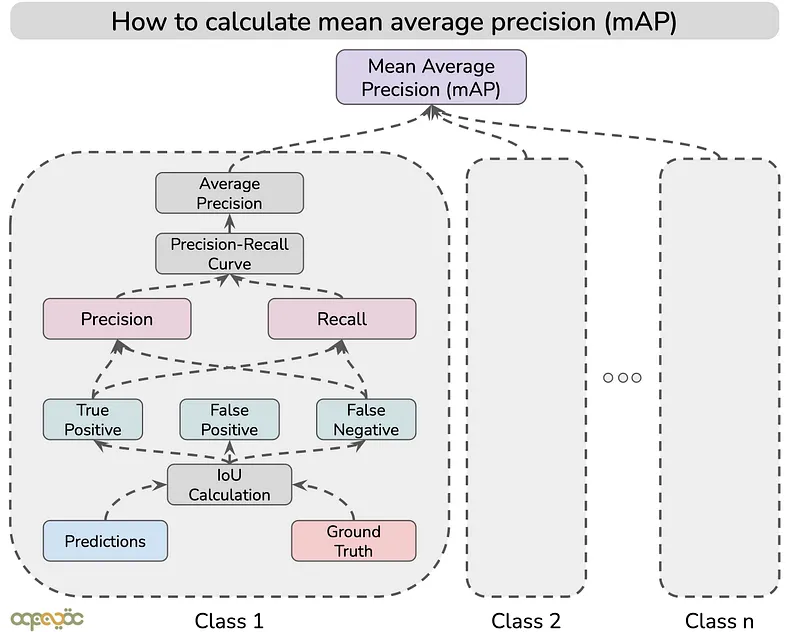
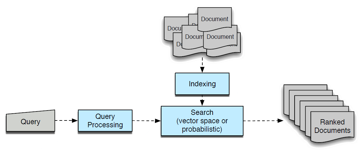
We use various metrics to measure the performance of a model in computer vision tasks involving object detection or re-identification (ReID). The most commonly used metric is Mean Average Precision (mAP). It gives a single overall score of a model's prediction accuracy across all object categories. 

The mAP is used in many benchmark challenges, such as the PASCAL Visual Object Classes (VOC) challenge, the COCO challenge, and others.

In this guide, we will cover:

1. Precision, recall, and the confusion matrix: Foundations of mAP
2. The precision-recall curve and average precision (AP)
3. AP vs. mAP: How to calculate mean average precision
4. Mean average precision in object detection
5. Why mAP? Advantages and considerations
6. Improving mAP: Tips and techniques
7. How to use Lightly AI to improve mAP

If you want to build your computer vision model with a high mAP score, then you need quality data for training. At Lightly, we help you optimize both the data and the model. 

• LightlyOne: Helps you select the most relevant data for training to reduce redundancy and improve mAP.
• LightlyTrain: Fine-tune models on curated data using self-supervised learning to boost performance.

You can try both for free to see how intelligent curation cuts labeling costs and to build image classifiers, object detectors, and semantic segmentation models with higher mAP.

Precision, Recall, and the Confusion Matrix: Foundations of mAP

We first need to know about precision and recall metrics to understand mAP. 

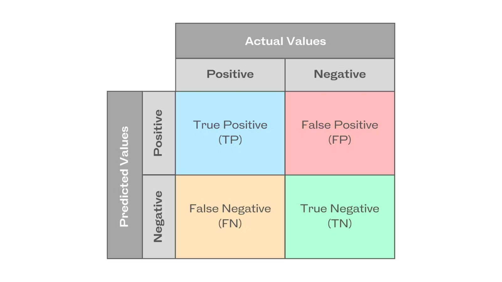
These two come from the outcomes of a model's predictions that are usually organized into a confusion matrix.

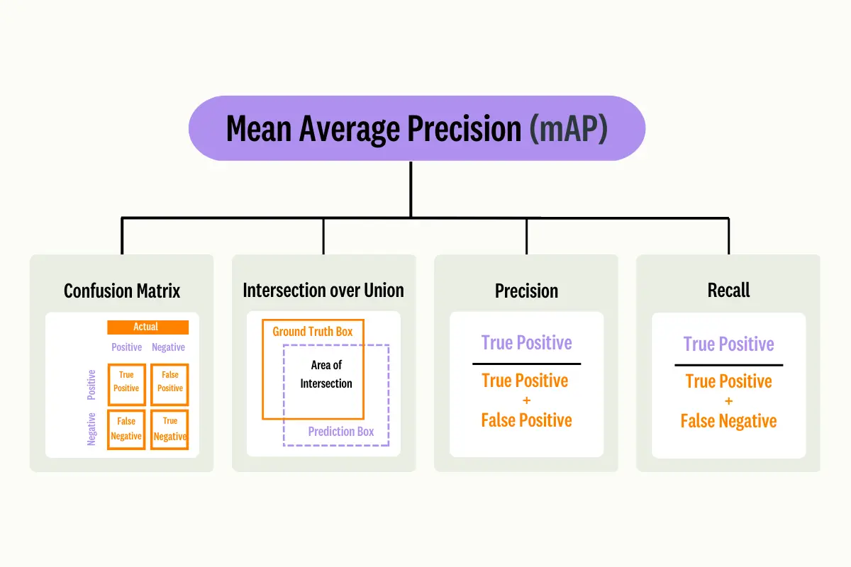
Confusion Matrix

A confusion matrix is a table that shows how accurately a machine learning model’s predictions match the ground truth. 

For a given class, there are four possible outcomes:

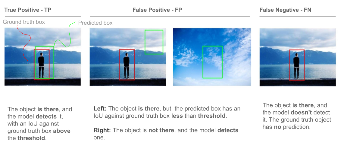
• True Positive (TP): The predicted label matches the ground truth.
• False Positive (FP): Predicted label does not match the ground truth (Type I Error).
• False Negative (FN): Model predicts a label, but it is not a ground truth label  (Type II Error).
• True Negative (TN): The model does not predict a label, but it is included in the ground truth.

In object detection, things are much more complex than a simple right or wrong. The detection model predicts the object in the image and also tells its position with a bounding box. 

We compare how much the predicted box overlaps with the ground truth box to decide if the model's prediction is correct using the Intersection over Union (IoU) metric.

Intersection over Union (IoU)

Intersection over Union (also called the Jaccard Index) measures the overlap between the predicted bounding boxes and the ground truth bounding boxes. 

It is calculated as a ratio of the overlap area (intersection) to the combined area covered by both boxes (union). 

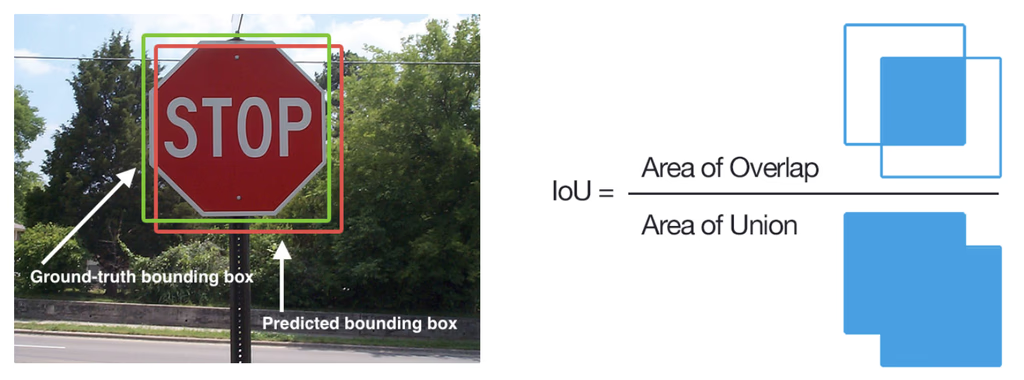
A higher IoU (closer to 1) indicates the predicted bounding box coordinates are more closely matched with the ground truth box coordinates, while an IoU near 0 means minimal overlap.

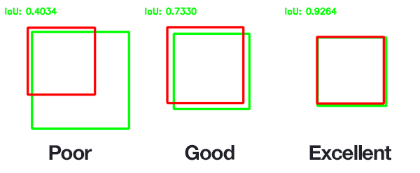
We calculate the IoU score for each detection and set a threshold to classify it. If a detection's IoU score is above the threshold, we classify it as a positive prediction. If it falls below, it is classified as a false prediction. 

Using the scores, we categorize the predictions as true positives, false negatives, and false positives.

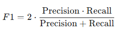
Precision (Positive Predictive Value)

Precision measures how accurate a model's positive predictions are. It is the ratio of correct positive predictions (TP) to the total number of positive predictions made (TP + FP). The precision formula is:

Recall (Sensitivity)

Recall measures how well the model finds all the actual positives. It is the ratio of correct positive predictions (TP) to the total number of actual positives (TP + FN). The recall formula is:

Let’s take an example to illustrate how recall and precision are calculated. Below are images showing objects with ground truth boxes on the left and predictions on the right, and the IoU threshold set to 0.5.

• When multiple boxes detect the same object, the box with the highest IoU is considered TP, while the other boxes are FP.

• If the object is present and the predicted box has an IoU < threshold with the ground truth box, the prediction is considered an FP. More importantly, because no box was detected properly, it also counts as an FN.

• If the object isn't present in the image but the model detects one, the prediction counts as an FP. 

Recall and precision are then computed for each class using the formulas above, by accumulating the counts of TP, FP, and FN.

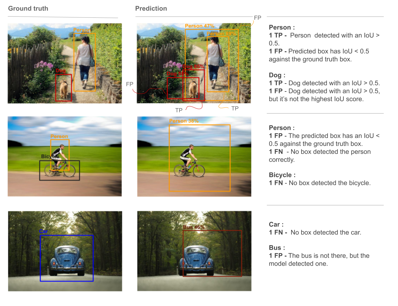
Let’s calculate recall and precision for the ‘Person’ category:

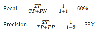
Now, if you’re not satisfied with those results, what can you do to improve the performance? You can often adjust a model's confidence threshold. 

But if you set a high confidence threshold, the model will only make predictions it is highly confident in. This usually leads to high precision but lower recall (it might miss some less obvious objects).

If the confidence threshold is set low, the model will make more predictions, even if it's not very sure. It can cause a high recall but lower precision. Because of this tradeoff, we use a precision-recall curve (PR curve) for a more complete view.

The Precision-Recall Curve and Average Precision (AP)

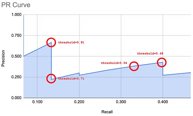
A precision recall curve is a graph that plots precision values (y-axis) against recall values (x-axis) at different confidence thresholds. 

You rank all your model’s positive predictions by their confidence scores to create the curve, then calculate precision and recall at each point.

A good model maintains high precision even as recall increases, so its PR curve stays near the top-right corner of the graph. A poor model's precision drops quickly as it tries to achieve higher recall.

The PASCAL Visual Object Classes 2012 (VOC2012) challenge uses the PR curve as a metric alongside average precision. It is a supervised learning challenge with labeled ground-truth images. The dataset includes 20 object classes such as person, bird, cat, dog, bicycle, car, chair, sofa, TV, bottle, etc.

The PR curve provides a clear visual summary, but the curve can be noisy, and its saw-tooth shape makes it difficult to estimate the performance of the model. 

Similarly, it can be hard to compare different models when their PR curves cross each other. Therefore, we calculate a single number called the Average Precision (AP).

AP - Average Precision

Average Precision (AP) is the area under the precision-recall curve. It shows the average of all the precision scores across different recall levels. A higher AP means the model gives better performance across all confidence thresholds.

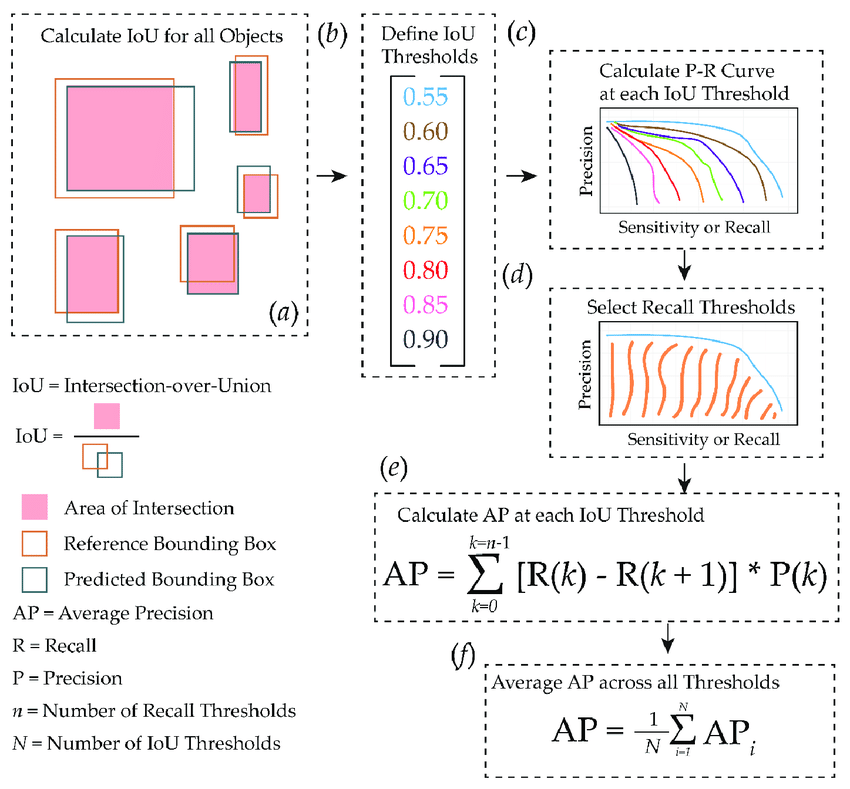
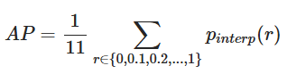
A common technique for calculating AP is 11-point interpolation (used in Pascal VOC competition). It involves averaging the maximum precision value for 11 spaced recall evaluation points (0.0, 0.1, 0.2, 0.3, 0.4, 0.5, 0.6, 0.7, 0.8, 0.9, 1.0). 

For each recall point r, find the highest precision p from all recalls r˜ ≥ r. Mathematically:

Where: 

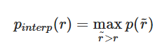
Where p(r˜) is the measured precision at recall r˜. 

Graphically, this is simply a way to smooth out the spikes from the graph and make it look like:

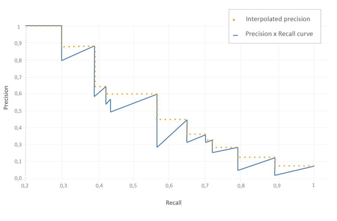
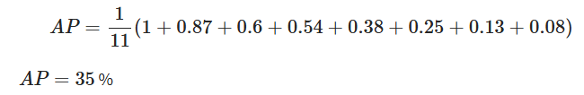
Let’s calculate the interpolated AP for all recall values using the p_interp formula, and though our recall levels start at 0.2, the strategy remains the same.

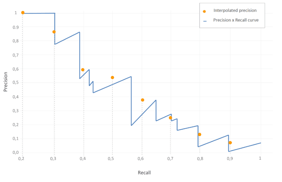
Now, calculate the average of all of the interpolated precision points.

The modern benchmarks use the 11-point interpolation method to calculate the exact AUC by considering all unique recall points, which provides a more precise AP value. This single AP score gives a strong way to evaluate a model's performance on a single class.

Other Metrics

In addition to the average precision, it's helpful to compare it with other evaluation metrics to better understand its benefits.

• F1-Score: It is the harmonic mean of precision and recall and provides a single score for both metrics, but only for a single confidence threshold. AP is a thorough overview as it summarizes performance across all thresholds.

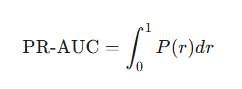
• PR-AUC (Area Under the PR Curve): PR-AUC is conceptually the same as average precision, and the terms are used interchangeably. But AP is a specific method, like 11-point interpolation for calculating the area under the PR curve.

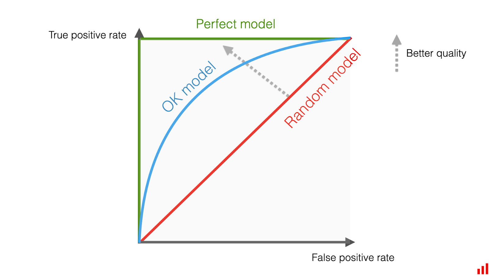
• ROC-AUC (Area Under the Receiver Operating Characteristic Curve): The ROC curve plots the true positive rate against the false positive rate. While useful for balanced classification problems, it is less informative for object detection or information retrieval. 

‍

Here is a summary of some of the key metrics above and how they relate to each other.

‍

How to Calculate Mean Average Precision

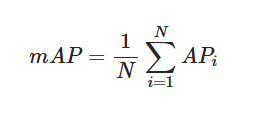
Once we grasp average precision, the concept of mean average precision (mAP) is quite simple. The mAP is calculated by taking the mean of the AP scores over all classes. If a dataset includes N different classes, you compute the AP for each class and then average them.

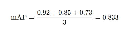
For instance, if you have a model for three classes (cat, dog, bird) and calculate their average precision to be:

• AP(cat) = 0.92
• AP(dog) = 0.85
• AP(bird) = 0.73

The mAP calculation would be:

Similarly, in the PASCAL VOC dataset, AP is computed for each of the 20 categories and then averages these to get the mean average precision.

Mean Average Precision in Object Detection

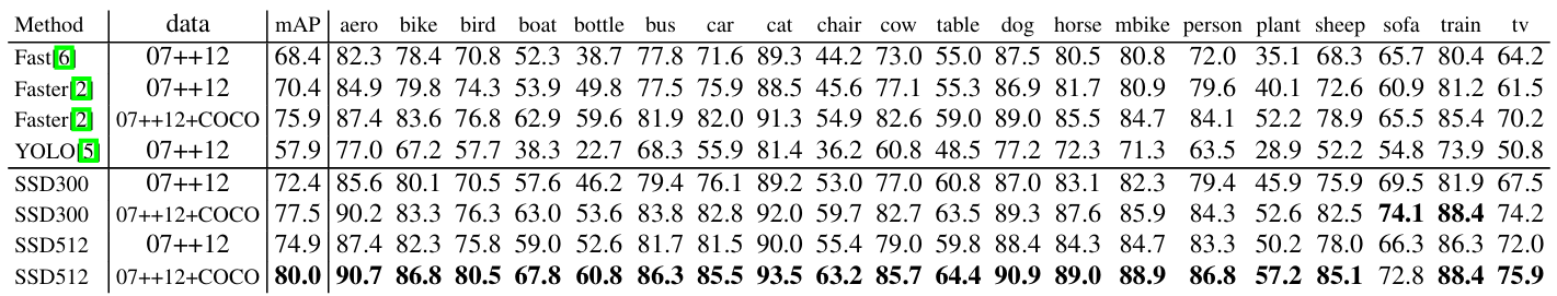
The mAP is a standard metric for evaluating object detection models. The object detection algorithms like YOLO, SSD, and Faster R-CNN are all evaluated based on their mAP scores.

Here is a summary of the steps to calculate mAP in object detection:

1. Get Predictions: Run the model on a set of test images to get all predicted bounding boxes, along with their class labels and confidence scores.

2. Match Predictions to Ground Truth: For each class, match the predicted boxes to the ground truth boxes using an IoU threshold to classify them as true positives or false positives. Any ground truth objects that were not detected are false negatives.

3. Calculate the PR Curve: For each object type, sort the predictions from most to least confident. Go down the ranked list and calculate the precision and recall at each step to create the points for the PR curve.

4. Calculate AP for Each Class: Compute precision for each class and recall to find the area under its PR curve. It gives you the average precision AP for that class.

5. Take the Mean of the APs: Calculate the mean of all the per-class AP scores, and the result is the mAP score for your model.

A higher mAP score indicates that the model is both accurate in its classifications and good at localizing objects. 

Different object detection benchmarks use slightly different ways to calculate mAP through varying the IoU threshold.

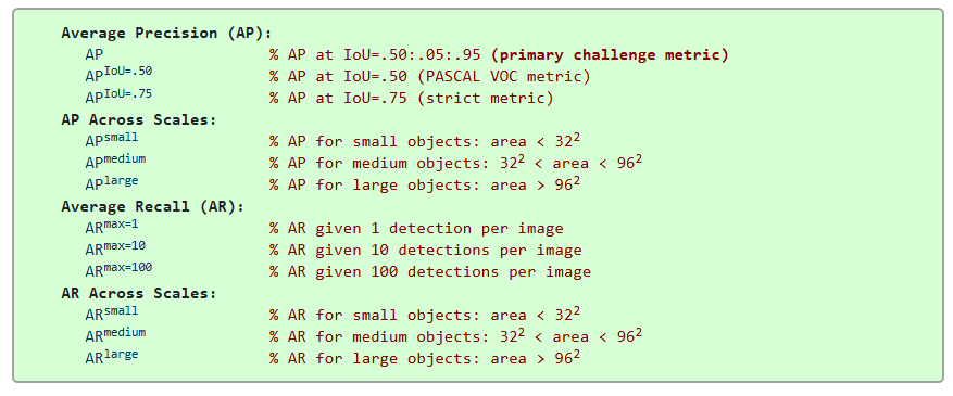
The PASCAL VOC challenge calculates mAP using a single IoU threshold of 0.5 (mAP@0.5). It uses an 11-point interpolated precision method for the AP calculation.

MS COCO challenge calculated mean average AP over 10 different IoU thresholds, from 0.5 to 0.95 in steps of 0.05 (mAP@[.5:.95]). This method rewards models that achieve high precision in localization.

Similarly, the Google Open Images dataset, used in the Google Open Image Challenge, also uses mAP@0.5 for its detection track, but over a much larger set of 500 classes.

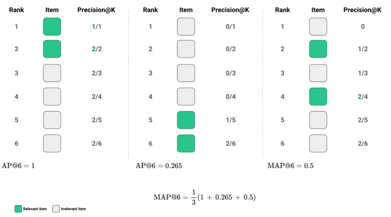
Mean Average Precision in Information Retrieval

So far, we are discussing the mAP in terms of object detection, but it is also a key metric in information retrieval. It assesses the effectiveness of search algorithms and recommendation systems. 

An information retrieval task involves a search system, like a search engine, where someone types in a query and it returns a list of documents ranked by relevance.

‍

Similar to object detection, mAP is calculated by averaging the average precision (AP) scores across multiple queries or search terms. 

AP in the information retrieval context is the average precision at different recall levels for a single query, considering only the relevant documents. A higher mAP means the system is better at retrieving relevant information at the top of the search results. 

Why mAP? Advantages and Considerations

Mean average precision is a go-to metric due to its numerous strengths for evaluating models in information retrieval and computer vision applications. However, it's also good to know its limitations. 

Advantages of mAP

Before diving into the drawbacks, first consider why mAP is so widely used.

• Thorough Evaluation of Model Performance: mAP summarizes the precision and recall into a single metric and provides a more informative view of model performance.
• Fair for Comparisons: Because it's threshold-agnostic, you can compare two models fairly without worrying if one was just tuned to a better confidence threshold.
• Sensitivity to Ranking Order: Simpler metrics determine the presence of relevant items within a certain cutoff, while mAP evaluates how well the system ranks these items. It helps models to place more relevant items higher in the predicted list. For example, a relevant search result that appears on the tenth page of results is technically "correct" but provides little practical value to a user. mAP effectively reflects this reduced utility by giving lower scores when relevant items are ranked poorly.

Limitations and Considerations of mAP

Keep the following limitations in mind to get a balanced understanding of the mAP role.

• Class Imbalance: Since mAP is an average across all classes, a high score can sometimes hide poor performance on a rare class in computer vision. It's always a good idea to look at the individual AP scores for each class.
• Human-interpretability: While precision and recall are easy to understand, the meaning of mAP (average area under a curve) can be confusing for non-specialists. For example, a score of "50% mAP" on the COCO benchmark is a good score, but it might not be immediately obvious to everyone.
• Sensitivity to IoU Threshold Selection: The mAP score is sensitive to the choice of the IoU threshold used to define a true positive detection. A model's precision value can change greatly depending on the IoU threshold. For example, an object detection might be correct at an IoU of 0.5 but incorrect at 0.8, even if the class prediction was accurate. The sensitivity means a model optimized for one threshold might not perform well at another.
• Computationally Intensive: For large datasets with millions of predictions, calculating the full mAP can take more time and computing power, too.

Tips and Techniques to Improve mAP 

Improving the model's mAP score is usually the primary goal in training. Here are some practical ways to do it:

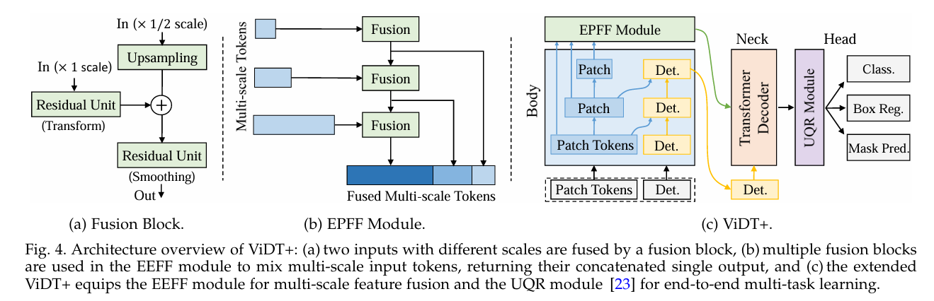
• Better Model Architecture: Use stronger backbones like ResNet, EfficientNet, or transformer-based detector heads to improve feature representation and enhance mAP. The paper ViDT (Vision and Detection Transformers) showed that a transformer-based detector achieves a maximum AP of 53.2 on COCO. 

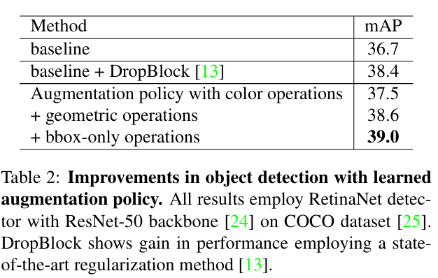
• Data Quality and Augmentation: More quality-labeled data is almost always better. Data augmentation creates more training variety by modifying the existing data and helps the model generalize, which leads to improved both precision and recall. The paper, Learning Data Augmentation Strategies for Object Detection, shows that a learned augmentation policy on COCO improved detection accuracy by more than +2.3 mAP.

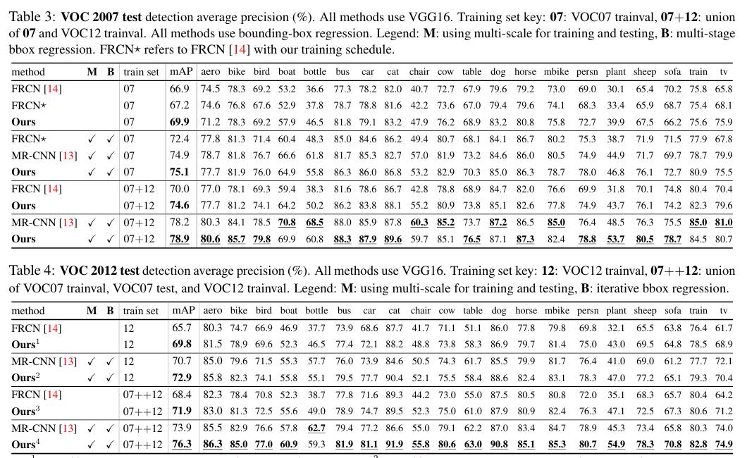
• Hard Negative Mining: Sometimes, a model gets confused by background patches that look like objects, and it creates false positives, which affects precision. Hard negative mining involves training the model on tricky negative examples to improve its ability to differentiate. The paper Training Region-based Object Detectors with Online Hard Example Mining showed that Online Hard Example Mining (OHEM) led the object detector to achieve top mAPs of 78.9% on PASCAL VOC 2007 and 76.3% on 2012.

• Tune Hyperparameters: Experiment with learning rates, optimizers, and other training settings. The right hyperparameters can have a big impact on the final mAP score.
• Use Pretrained Models: Starting with a model that has been pretrained on a large dataset (like COCO or ImageNet) and then fine-tuning it on your own data is a very effective strategy.
• Active Learning and mAP: Actively selecting additional training data when the model is uncertain or makes mistakes can greatly improve mAP for the next round of training. Use an intelligent platform like Lightly AI in your ML pipeline to select data through active learning, pretrain, and fine-tune the model iteratively to improve the mAP.

How To Use Lightly AI To Improve Mean Average Precision

Improving the model mAP score requires starting with better training data, not just in quantity, but in relevance. Raw data can be huge and contain a lot of repetitive or easy examples that don't help the model learn and add extra labeling costs, too.

We can use the LightlyOne platform to pick the most informative and varied samples that help raise mAP. It cuts out redundancy and focuses on underrepresented examples by using visual embeddings and self-supervised learning.

Using only quality data for training, LightlyOne helps reduce false positives and false negatives, which improves average precision for each class.

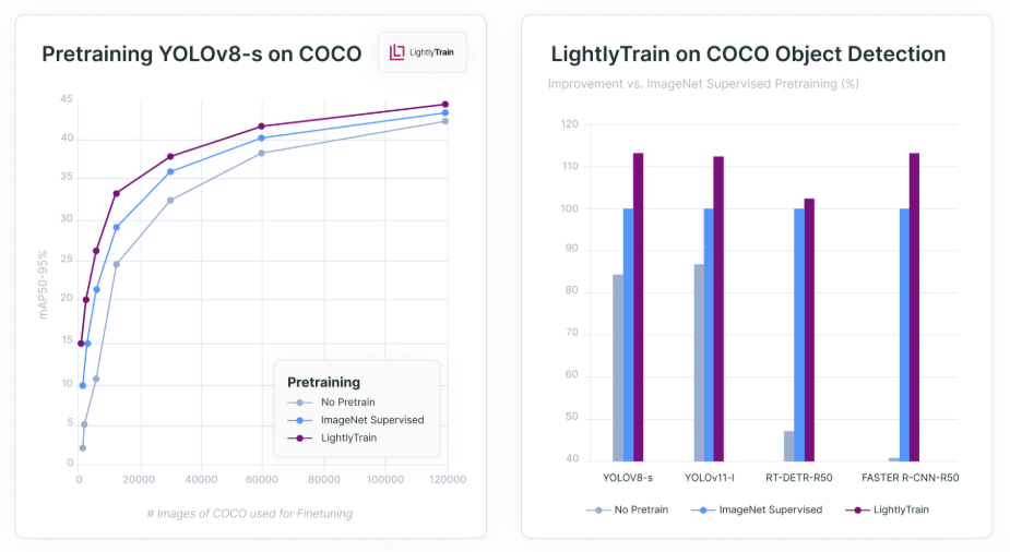
Instead of starting from scratch, we can use LightlyTrain to pretrain our own vision models on the unlabeled data selected from LightlyOne. It performs better than models that start from pre-trained ImageNet weights or are trained from scratch. 

LightlyTrain achieves up to 36% higher mean average precision (mAP) in spotting objects compared to traditional training methods. 

In the object detection use case, Lightly AI helped AI Retailer Systems reach 90% of their maximum mAP using only 20% of the training data.

Conclusion

Mean average precision (mAP) is the current standard performance metric and brings clarity to evaluating computer vision models. It provides a single score that combines the accuracy of predictions (precision) with the ability to detect all relevant items (recall).

You can better assess your models and make smarter training choices by understanding how mAP works. Although it has its complexities, mAP is a valuable tool for developing more accurate and robust computer vision systems.