‍

Introduction

When we talk about prediction using machine learning (ML) models, it’s important to understand prediction errors. The model shows three types of error: bias, variance, and irreducible error (noise). 

We strive to minimize bias and variance to create a model that can accurately predict on unseen data.

In this guide, we'll cover:

1. What bias in ML really means (high vs. low bias)
2. What variance is and how it affects your model
3. Practical techniques to balance bias and variance
4. How different algorithms inherently juggle bias and variance
5. How Lightly AI helps manage the bias-variance tradeoff

Building an ML vision model for a specific problem requires quality training data and smart strategies to manage the bias-variance tradeoff. We at Lightly help reduce bias and control variance through:

• LightlyOne: Curate the most representative and diverse samples from your training dataset to reduce variance and improve generalization, avoiding overfitting.
• LightlyTrain: Pretrain and fine-tune models with stronger pattern recognition to lower bias and capture underlying patterns effectively.

You can try both for free!

What is Bias in Machine Learning? (High Bias vs. Low Bias)

In machine learning, bias refers to a systematic error that arises when a learning algorithm makes wrong assumptions about the data. It causes the model's predictions to deviate from actual values most of the time.

Simply put, bias measures how far off the model’s predicted values are from the actual values on average. 

To quantify bias, consider a true parameter value A and its estimator, Â, derived from data points. Then, the bias is calculated as:

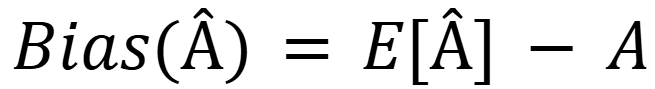
Where E[Â] is the expected value of the estimator across different samples.

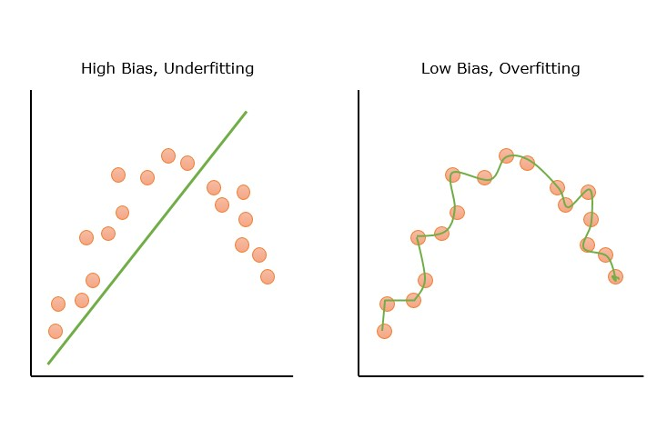
High Bias (Underfitting)

A high bias or very simplified model does not fit the training data well. It makes erroneous assumptions about the relationship between input features and the output. 

Since its assumptions are too rigid, the high-bias model fails to find the underlying patterns in the training dataset.

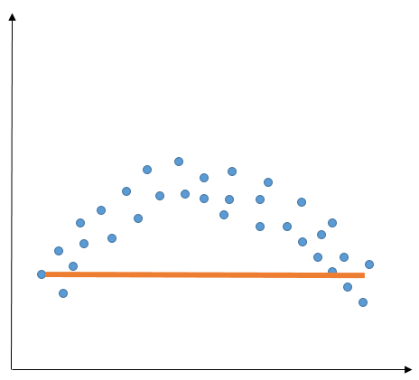
For example, when you're trying to draw a straight line through data points that actually follow a curve, no matter how you move the line, it won't fit well. 

The straight line is your simplified model, and its failure to follow the curve is its bias.

Low Bias

A model with low bias makes fewer assumptions about the data. It adapts well and can easily identify complex underlying patterns in training data. 

At first glance, low bias seems perfect, as it means the model learns everything well. 

But, aiming for zero bias is not always good. If a model is too flexible, it can also learn the random noise in the training data, including irrelevant information, which can lead to overfitting. 

This can result in the model performing poorly on new data.

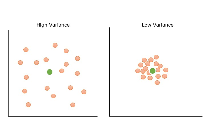
What is Variance in Machine Learning? (High Variance vs. Low Variance)

Variance in ML refers to the model’s sensitivity to fluctuations in the training data. 

More specifically, it measures how much the model’s predictions would vary if we trained it on different subsets of the data. Mathematically, variance is expressed as:

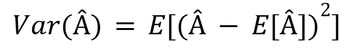
Where  is the predicted value and E[Â] is its expected value averaged over multiple training sets.

High Variance (Overfitting)

A high variance model is often an overly complex model that has learned the genuine patterns and also the random noise in the training data. It leads to overfitting.

These high-variance models fit the training data almost perfectly and show high training accuracy but low test accuracy.

Low Variance

A model with low variance produces nearly similar predictions regardless of the training data it sees. A low-variance model is unable to capture the hidden pattern in the data and eventually leads to underfitting. 

Low variance mostly occurs when we have a small amount of data or use a simplified model, like linear regression (which tends to have low variance).

Pro Tip: Both high and low variance issues often stem from poor data quality, whether it's noisy samples or lack of diversity. Check out our guide to data curation to learn how smart data selection can help optimize model performance.

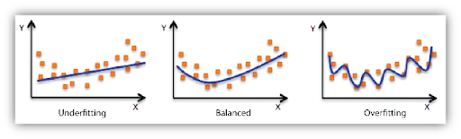
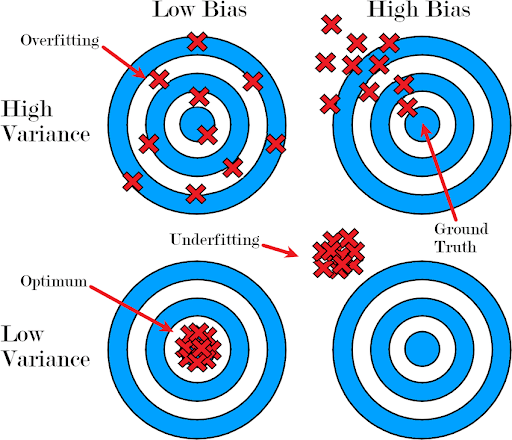
Underfitting vs Overfitting: Too Simple vs Too Complex Models

The challenge we face in building models is to find the right level of complexity. If our model is too simple, it won't capture enough information (underfitting). If it's too complex, it will pick up on random noise rather than the actual pattern (overfitting).

Our goal is to find a balance where the model learns the right signals from the training data without being misled by the unimportant details (random noise).

The table below will summarize the differences between underfitting and overfitting in terms of model behavior and errors:

‍

Now that we’ve defined bias and variance individually, let's put them together and see how they interplay.

The Bias-Variance Tradeoff

The bias-variance tradeoff is the root compromise we face when building and tuning machine learning models. 

It highlights that we cannot lower both bias and variance to zero in parallel. Improving one often comes at the expense of the other.

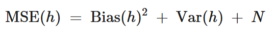
To grasp the tradeoff, consider the total prediction error for any predictive model, which can be thought of as the sum of three parts:

• Bias²: The squared error from wrong assumptions. We square it to get the positive value, since the error can not be negative.
• Variance: The error from sensitivity to data fluctuations.
• Irreducible Error (Noise): This is the natural level of randomness (noise) in the data. No matter how good our model is, we can never completely remove this error. It’s caused by factors like measurement errors or hidden variables that affect the data but are not included in our features.

Relationship is of the above three, famously written as:

Since we can't do anything about the irreducible error (fixed and beyond our control), our focus in machine learning is to find a model that minimizes the sum of bias-squared and variance. 

Practically, we often start with an underfit model and gradually increase complexity until we start to see overfitting. Then dial it back or apply techniques to control variance. This balance is the essence of the bias-variance tradeoff. 

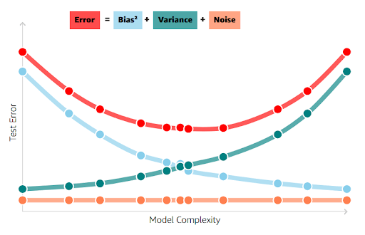
Let's visualize how tradeoff behaves as model complexity increases. 

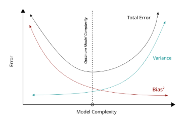
In the above image, in the low-complexity regime (far left side), the model is too simple, resulting in a high bias and low variance.

At a moderate level of complexity, the bias has decreased to an acceptable level, and the variance hasn't increased too much yet. This point is close to the best possible test error, the bottom of a U-shaped curve.

In the high-complexity regime, making the model more flexible yields very little reduction in bias (it’s already near zero on training data) but greatly increases variance.

Bias-Variance Decomposition: The Math Behind the Tradeoff

Trading off bias and variance improves predictive accuracy, and it is typically introduced through the decomposition of mean squared error (MSE).

Let's understand the derivation of MSE in terms of bias and variance, starting with an example prediction task. 

Predicting the exact volume of ice cream that will be consumed in Rome next summer is quite tricky. But it's easier to say that more ice cream will be eaten next summer than next winter. 

Although hotter weather generally increases ice cream sales, we don't know the exact link between daily temperatures in Rome and ice cream consumption. 

To predict how temperature (X) affects ice cream consumption (Y), we use a method called regression analysis, which looks at the relationship between these two factors.

Suppose we predict that the value of Y is h. How can we tell if our prediction is good?

Generally, the best prediction is the one that is closest to the actual Y. If we don't care about whether our errors are too high or too low, we often measure the accuracy by looking at the square of the difference between Y and h, which is:

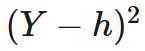
Since the values of Y vary, we consider the average value of (Y-h)^2 by computing its expectation, E [((Y-h)^2)]. This quantity is known as the mean squared error of h. 

Consider we want to predict Y using some data D that shows the relationship between X and Y, like last year’s daily temperatures and ice cream sales in Rome. We refer to our prediction as h(X) to represent this concept.

We aim to minimize the average squared error, which can be expressed as E[(Y−h(X))^2]. Since the value of Y is directly related to the value of X, it's more precise to evaluate our prediction by looking at the average error for each possible value of X.

For each specific value, x, the best possible prediction for Y is its average value, given that X = x. This is referred to as the conditional mean, E[Y| X = x]. 

This ideal, true relationship is what we call the regression function, r(x), which gives the optimal value of Y for each value of x:

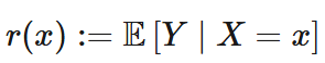
Although the regression function represents the true population value of Y given X, this function is usually unknown and often complex. For this reason, we approximate it with a simplified model or learning algorithm, h(⋅). 

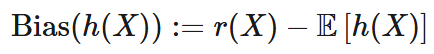
The bias is the difference between the true relationship, r(X), and the average prediction of our model, E[h(X)], over all possible datasets.

Variance measures the average deviation of a random variable from its expected value. We compare the predicted value h(X) of Y based on a dataset D to the average prediction of the model across all possible datasets, E[h(X)]. We express this variance as:

‍

We can now derive bias-variance decomposition by starting with the MSE and adding and subtracting the expected value of our model's prediction.

Let h refer to our estimate h(X) of Y, r refer to the true value of Y, and E[h] the expected value of the estimate h (taken over all possible datasets). Then,

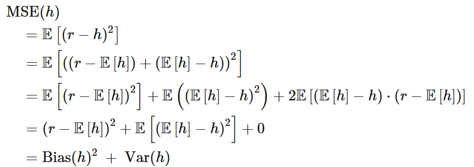
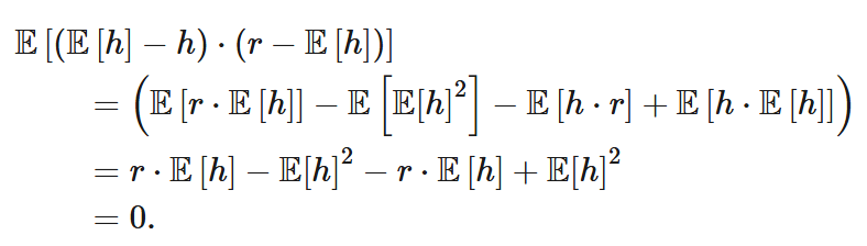
Where the third term is zero, since

Finally, the prediction error of h(X) due to noise, N, which occurs independently of the model or learning algorithm, adds irreducible error. 

Thus, the full bias-variance decomposition of the mean-squared error is:

Strategies to Balance Bias and Variance (Improving Model Performance)

Since both extremes lead to poor predictive accuracy, addressing them is crucial for the model's performance on unseen data. Below, we outline practical strategies using established methods to reduce bias or variance while minimizing total error.

First, let's review strategies for high bias.

How to Fix High Bias (Underfitting)

If your model is underfitting, it means it's too simple. You need to give it more power to learn the underlying patterns. Some strategies are:

• Increase Model Complexity: Switch to a more powerful algorithm. If you are using linear regression for non-linear data, try polynomial regression, a Random Forest, or a Gradient Boosting model. For neural networks, you can increase the number of layers or the number of neurons per layer.
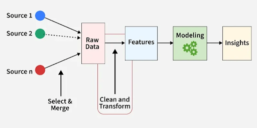
• Add Features (Feature Engineering): Sometimes, the issue is that the model lacks sufficient information to make good predictions. You can provide more context by creating new features from the existing ones or adding new data sources.

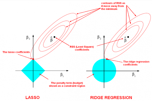
• Decrease Regularization: Regularization techniques like Ridge (L2), Lasso (L1), or others impose penalties that tend to simplify the model (to prevent overfitting). If your model already has high bias, you might be over-penalizing it. Try reducing the regularization hyperparameter (often called lambda or alpha) to give the model more flexibility.
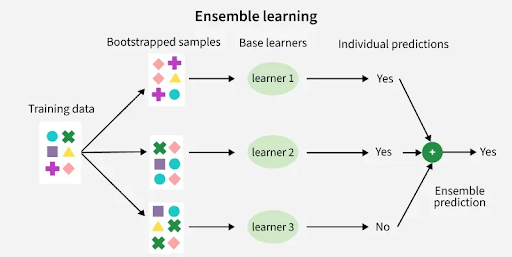
• Ensemble Methods: Ensemble approaches like bagging, boosting, and random forests combine multiple models to reduce variance without increasing bias. For instance, bagging reduces overfitting by averaging predictions across several models, while boosting sequentially improves weak learners to reduce bias.

How to Fix High Variance (Overfitting)

If your model is overfitting, it's too complex, or it has learned the noise in your data. You need to either simplify it or provide it with better data.

• Get More Training Data: The most effective way to reduce variance is by increasing the size or diversity of the training dataset. But when you are working on a computer vision model, getting quality data in large quantities is expensive. You can then use active learning, which intelligently selects the most informative new data points to label. Lightly offers a tool, LightlyOne, that helps you scale active learning and reduce data and labeling costs.
  

• Simplify the Model: If the model is too complex, consider using a simpler algorithm or fewer parameters. For decision trees, you can prune the tree by limiting its maximum depth or setting a minimum number of samples required to make a split. For neural networks, reduce the number of layers or neurons.
  
  
• Use Regularization Techniques: Regularization adds a penalty to the model's loss function for being too complex, discouraging it from fitting noise.
  
  • L1 (Lasso) and L2 (Ridge) regularization add a penalty based on the size of the model's coefficients, effectively shrinking them. L1 can even shrink some coefficients to zero, performing automatic feature selection.

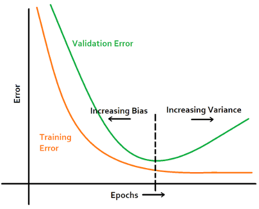
• Early Stopping is another regularization type; you can monitor the model's performance on a validation set. And stop the training process when the validation error stops decreasing and starts to rise, even if the training error is still going down.

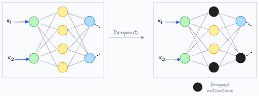
• Dropout (in neural networks) randomly deactivates a fraction of neurons during each training step. It forces the network to learn redundant representations and prevents it from relying too heavily on any single neuron.

• Feature Selection and Dimensionality Reduction: If you have too many features, your model might be learning from irrelevant or noisy ones. You can reduce the complexity of the problem and lower the model's variance by selecting only the features that matter.

Bias and Variance in Different Algorithms (Comparative Overview)

Different ML algorithms tend to have certain bias and variance based on their design and assumptions. 

For example, simple models like linear regression focus on stability but may not handle complex data well, which can lead to bias. 

On the other hand, more flexible models like decision trees can fit data closely, reducing bias but increasing the chance of overfitting, which leads to high variance. 

Knowing these tendencies helps you choose the right starting point for your problem. 

Below, we will compare different algorithms and see how they juggle the bias-variance tradeoff.

‍

Modern Perspectives: The Double Descent Phenomenon

For decades, the U-shaped curve was the accepted truth about the bias-variance tradeoff. But  with the rise of large models like deep neural networks, researchers have noticed a new pattern called double descent.

Sometimes, as you continue to increase model complexity past the point where it starts to overfit, the test error can surprisingly start to decrease again. The error curve goes down, then up (the classic "U" shape), and then back down.

Let's look at double descent more clearly with the help of graphs.

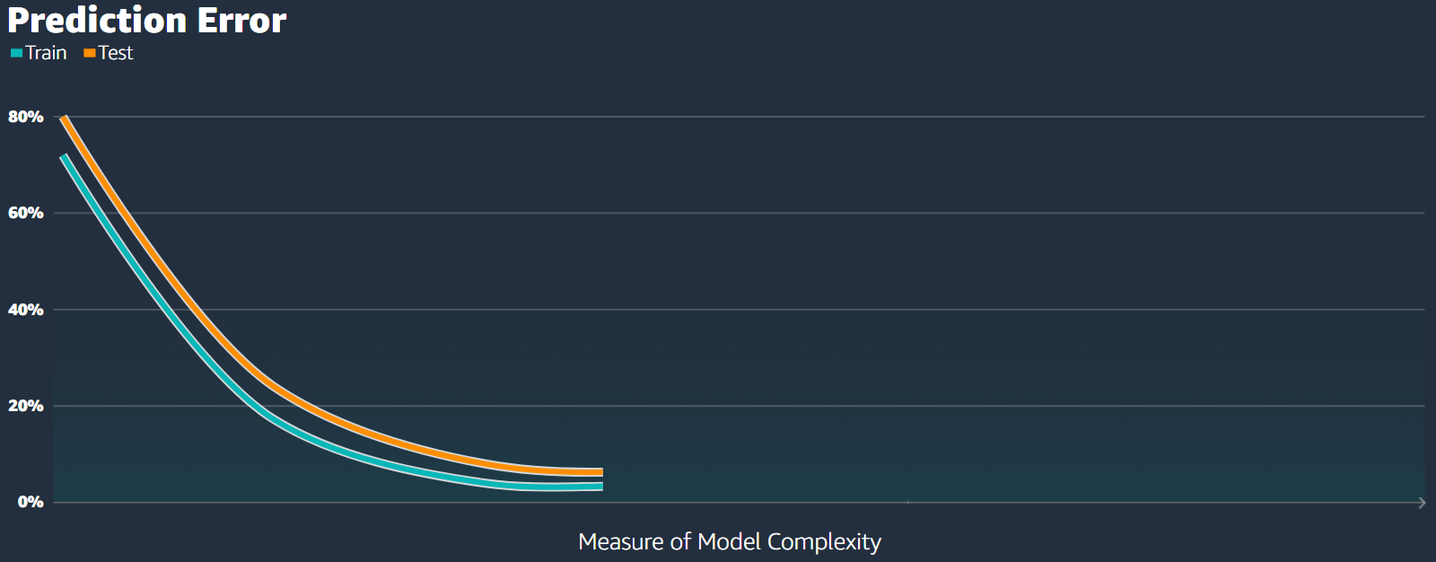
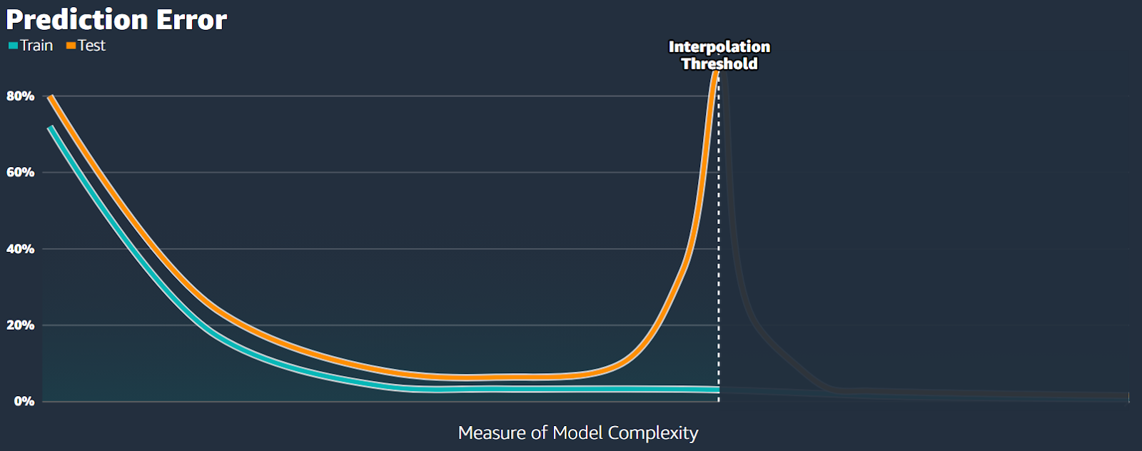
When we plot the training and testing errors against some measure of model complexity (like training time), they usually both decrease. The testing error tends to stay just a bit higher than the training error (see Fig.15).

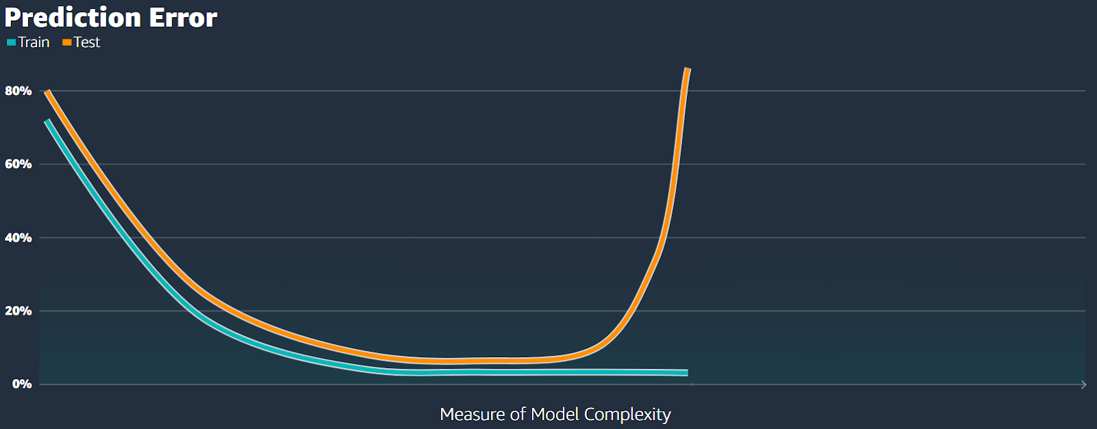
Under the classical bias-variance tradeoff, as the complexity of our model increases (moving right along the x-axis), we tend to overfit. The error on the test data becomes very large, while the error on the training data continues to decrease (see Fig.16).

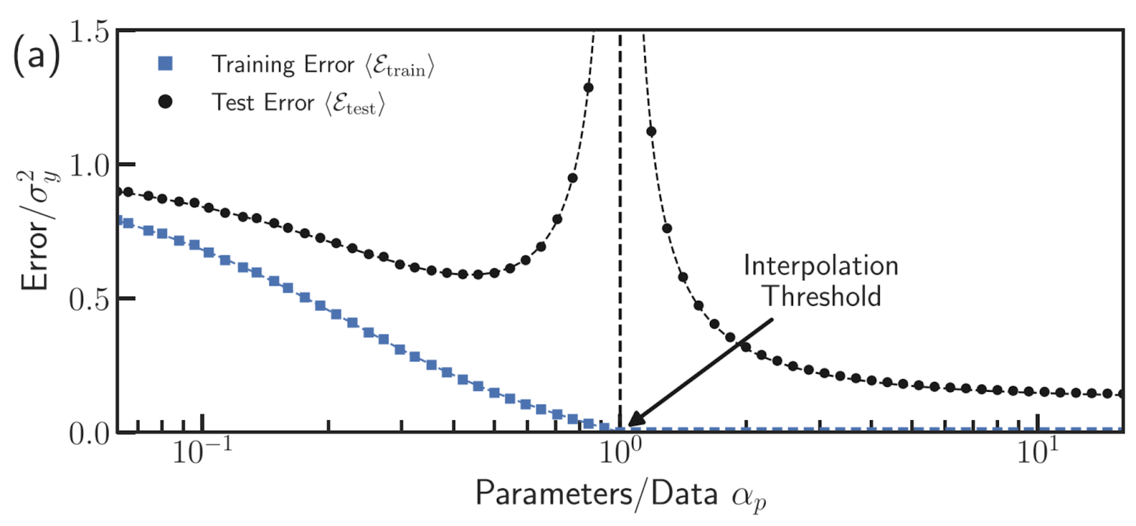
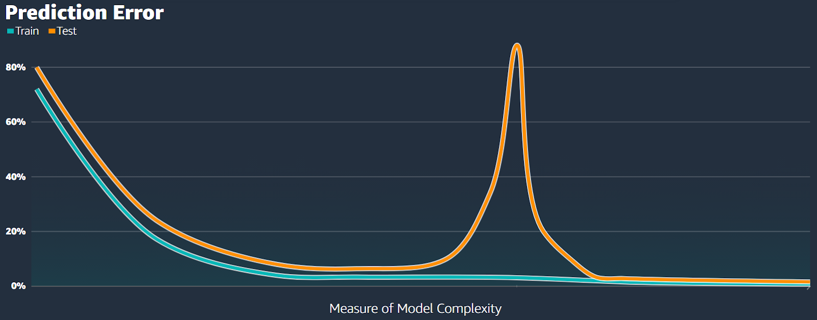
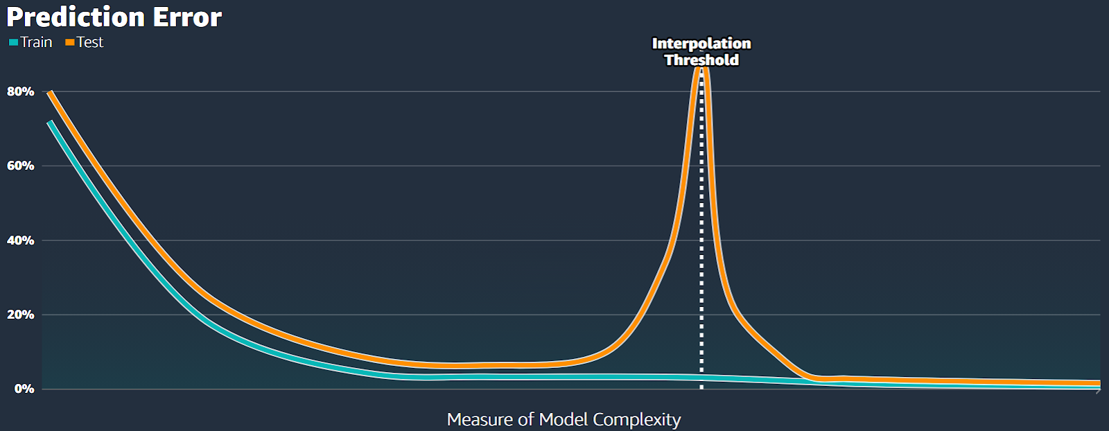
However, what we're seeing is a bit different. The error initially shoots up, then decreases to a new low point (see Fig.17). 

It means that even though our model is highly overfitted, it still achieves its best performance during this second decrease in error, which is why it's called double descent.

We refer to the area on the left side of the second decrease in error as the classical regime, where the model has too few parameters (see Fig.18). 

The point where the error is highest is called the interpolation threshold. 

In this classical regime, the relationship between bias and variance behaves as expected, with the test error forming the usual U-shaped curve.

To the right of the interpolation threshold, there's a behavior change. We call this area the interpolation regime (see Fig.19). 

How Lightly AI Helps Manage the Bias-Variance Tradeoff in Computer Vision Models

Achieving a good balance between bias and variance in computer vision models requires high-quality, varied data. 

These help the model learn important data features without becoming too specific or too general.

Lightly AI offers tools to help with these challenges. They assist in reducing both underfitting and overfitting in vision tasks.

LightlyOne helps curate the most representative and diverse samples from large training datasets using active learning and embeddings. 

It reduces variance, prevents overfitting by focusing on informative, non-redundant data, and improves unseen data performance, which lowers prediction error.

Once you have the desired data, you can then use LightlyTrain to train the model. It uses self-supervised learning to learn from unlabeled, domain-specific data. 

LightlyTrain improves the model’s ability to recognize patterns and adapt to real-world complexities. Eventually, leads to more accurate predictions and a better balance between underfitting and overfitting.

• LightlyOne Documentation: https://docs.lightly.ai/
• LightlyTrain Documentation: https://docs.lightly.ai/train/

Conclusion

Bias and variance are the twin pillars of error in ML models. Understanding their tradeoff is essential for building models that generalize well. 

High bias in ML models leads to oversimplification that miss patterns, while high variance causes models to memorize noise and fail on new data. 

With the right strategy and data tools, managing the bias-variance tradeoff becomes less of a struggle and more of a structured path to better predictions. Illustrating the phenomenon of double descent.

‍