‍

Introduction

If you’ve ever worked on computer vision tasks like object detection or image segmentation, you have likely run into Intersection over Union (IoU), commonly called Jaccard's Index. It gives a single overall score of a model's localization accuracy.

IoU plays a crucial role in many computer vision applications, including autonomous vehicles, medical imaging, and security systems.

In this guide, we will cover:

1. What is intersection over union?
2. How to calculate IoU
3. IoU role in object detection and image segmentation
4. Advanced IoU metrics
5. IoU in practice: Tips, tricks, and active learning applications
6. How Lightly AI improves IoU in computer vision models

Getting high IoU scores depends on the quality of the data you put into the training and the model's tuning. At Lightly, we help you improve both the data and the model.

• LightlyOne: Curate the most diverse and informative samples for training to reduce redundancy and improve localization accuracy.
• LightlyTrain: Pretrain and fine-tune models on curated data to maximize performance and achieve better IoU metrics.

Whether you're building object detectors or segmentation models, Lightly makes the process faster, smarter, and easier.

What is Intersection Over Union (IoU)?

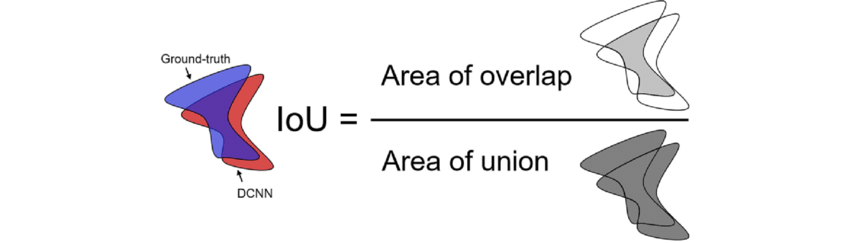
Intersection over union is an evaluation metric that quantifies the overlap between two regions. In the case of object detection and segmentation, these regions are the ground truth (the correct, hand-labeled area) and the predicted region from the model.

Simply put, IoU measures how well the prediction and ground truth agree on the area of the object.

‍

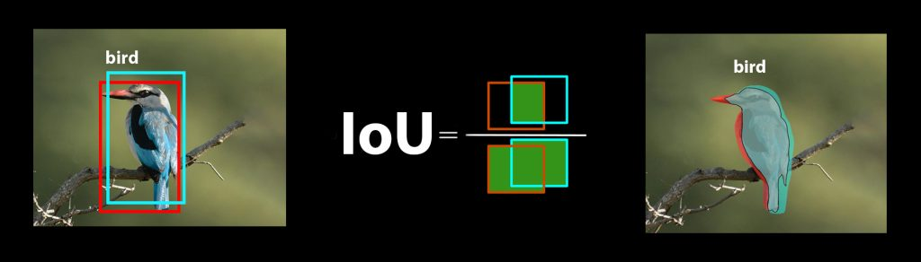
We calculate the IoU by putting the overlap area (intersection) in the numerator and the combined area covered by both boxes or masks (union) in the denominator. 

Mathematically:

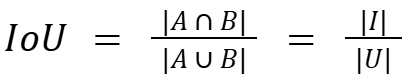
Where A and B are the prediction and ground truth bounding boxes or masks, I denote the intersection area, and U is the union area.

This ratio produces a value between 0 and 1:

• If the IoU = 1, the predicted box exactly matches the ground truth bounding box.
• When IoU = 0, there is no overlap at all.
• Intermediate values like 0.5 or 0.75 show that the boxes partially overlap.

Object detection consists of two sub-tasks: 

• Localization: Finding the location of an object in an image.
• Classification: Naming a class for that object.

But IoU focuses purely on localization. It only cares about how well the box was placed, not the object's class.

Let's look at a simple example. Suppose an image has a ground truth box for a cat with an area of 1000 pixels. If our model predicts a box overlapping 800 pixels of the ground truth (intersection), and the total area of the predicted box plus the ground truth (union) is 1200 pixels, then we calculate IoU:

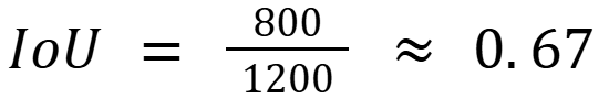
An IoU value of 0.67 shows a fairly good overlap, indicating that the model’s localization is close to the ground truth.

Ground Truth Data and Bounding Box Annotations

Ground truth data refers to verified, true data used to teach, validate, and test machine learning algorithms.

In computer vision, the IoU metric depends on the accuracy of this ground truth data (labeled data) when comparing results. If the ground truth annotations are wrong or inconsistent, even a perfect model will receive misleading IoU scores.

That’s why creating quality annotated datasets matters most in any vision project. It starts with curating good raw data that covers enough scenarios, including different object scales, angles, and lighting conditions.

LightlyOne helps curate raw data better in the quantity we want, and helps save time, effort, and annotation costs.

We can use the LightlyOne Selection feature to choose data using different strategies, such as DIVERSITY, TYPICALITY, or the BALANCE strategy to focus on specific classes.

Here’s a sample code example of configuring a LightlyOne selection. For more details, see our complete guide for common selection use cases.

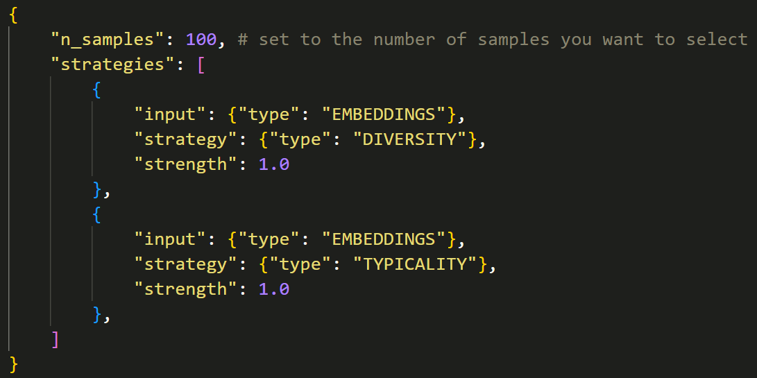
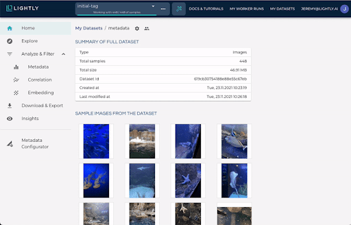
You can view and explore the selected dataset interactively on the LightlyOne Platform.

Once you have quality raw data, you can start labeling each object in the image (assigning a bounding box) that you want the model to detect. This process is called annotation or labeling. Labeling is usually done with specialized labeling software.

Annotation Tools and Sources

There are many data annotation tools available, and you can choose the one that best fits your needs. 

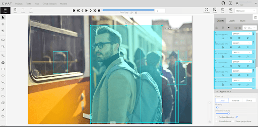
Software like LabelImg, CVAT, or commercial platforms such as V7 Darwin and Encord help in creating ground truth bounding boxes through manual labeling. 

Some of these tools use AI-assisted labeling, but human-verified ground truth is necessary for evaluation. 

Ensuring the ground truth is error-free is crucial since the IoU scores will show them as errors in the model.

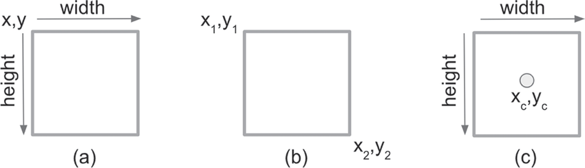
Annotating an image involves specifying the object's location using four numbers that represent its bounding box coordinates. 

There are two common formats for this:

• (x1, y1, x2, y2): This format, used by Pascal VOC, gives the coordinates of the top-left corner (x1, y1) and the bottom-right corner (x2, y2).
• (x, y, w, h): COCO uses this format, which gives the coordinates of the top-left corner (x, y), the bounding box's width (w), and the box's height (h).

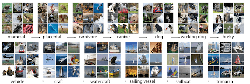
We can also get ground truth from public datasets like COCO (Common Objects in Context), Pascal VOC, or ImageNet, which provide pre-annotated images with bounding boxes. 

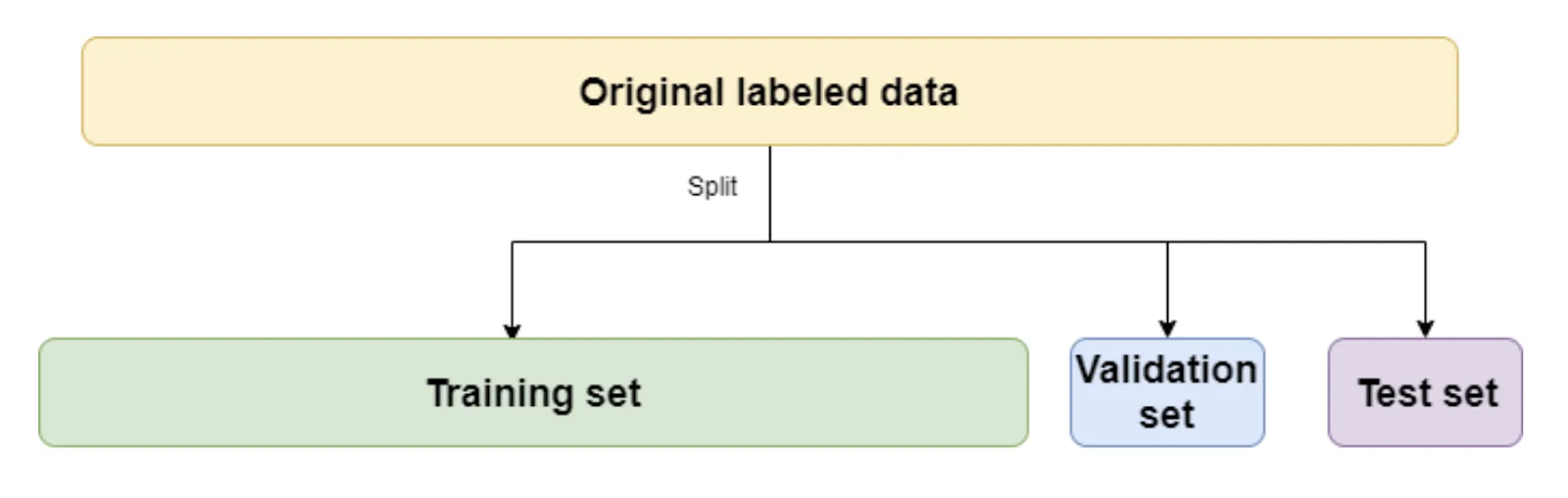
Dataset Splits (Train/Validation/Test) 

After annotating, split your data into a training and testing sets and a validation set.

The training set usually makes up 70-80% of the total data, validation 10-15%, and testing 10-15%. 

Separation ensures that when we calculate IoU scores on the test set, we assess the model's ability to handle new data, not just recall what it has already seen in training.

How to Calculate IoU: Step-by-Step

Now that we understand the concepts of IoU, let's dive deeper into its calculation. Assume we have two boxes, A and B, with corners marked by superscripts. Each box is defined by its upper-left (x0, y0) and bottom-right (x1, y1) corners. 

First, let's calculate the Intersection area.

The image below shows how we can find the upper-left (x0^I, y0^I) and bottom-right (x1^I, y1^I) corners of the intersection between two overlapping boxes. A superscript I indicates the intersection area.

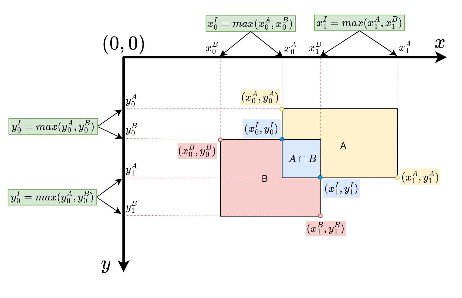
So, the coordinates of the intersection rectangle are as follows:

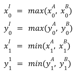
Then, we can calculate the intersection area as follows:

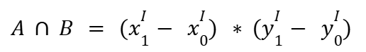
Let’s now calculate the union area. The union of two bounding boxes equals the sum of their areas minus the intersection area.

Where:

Finally, we can calculate the IoU as follows:

Here is a simple Python implementation of the steps above. This source code makes the logic clear.

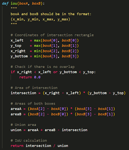
For practical applications, you would often use a vectorized Numpy implementation to compute IoUs for thousands of boxes at once, which is much more efficient.

IoU in Object Detection: Evaluation Metric and Thresholds

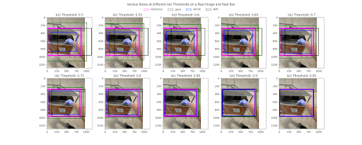
Now that we can calculate IoU for any pair of boxes, to evaluate an object detection model, we use an IoU threshold. This is a key step for benchmarking various object detection algorithms.

An IoU threshold is a cutoff value (between 0 and 1) that we choose to decide if a detection is correct or not. 

For a given predicted bounding box, we compare it to the corresponding ground truth bounding box.

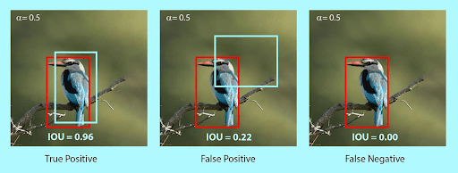
• If IoU >= threshold, we classify the prediction as a True Positive (TP). It means the model correctly found the object at the right position.
• If IoU < threshold, we classify it as a False Positive (FP). The model made a prediction, but it was too inaccurate to be considered correct.

Other types of errors also count as False Positives, such as predicting an object where there is none, or detecting the same object as a duplicate. A False Negative (FN) occurs when there is a ground truth object in the image, but the model fails to detect it.

‍

Using these TP, FP, and FN counts, we calculate Precision and Recall:

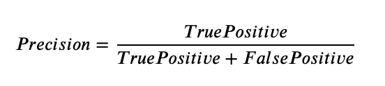
• Precision: It measures how many correct detections the model made. It is the ratio of correct positive predictions (TP) to total positive predictions (TP + FP). 

• Recall: It measures how many of the true positive cases the model actually finds. It is the ratio of correct positive predictions (TP) to all actual positives (TP + FN).

If we make our model more sensitive, it might find more objects (higher recall) but also make more mistakes (lower precision). The IoU threshold directly affects this, as a low threshold (such as 0.3) favors recall with more TPs, while a high threshold (0.8) favors precision with fewer TPs.

To avoid this trade-off, we use Average Precision (AP) to get a single number that sums up the model's performance across all thresholds. Mathematically:

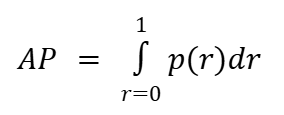
Where p(r) is the measured precision at recall r.

AP is the area under the Precision-Recall curve (PR curve). A higher AP means the model maintains high precision even as recall increases. 

In most datasets, we have multiple object classes. We calculate the AP for each class individually. Then calculate the mean Average Precision (mAP), which is simply the average of the AP scores across all classes.

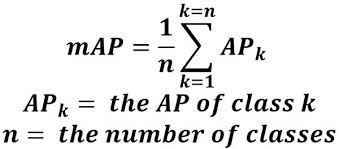
mAP is the most important evaluation metric for object detection benchmarks. 

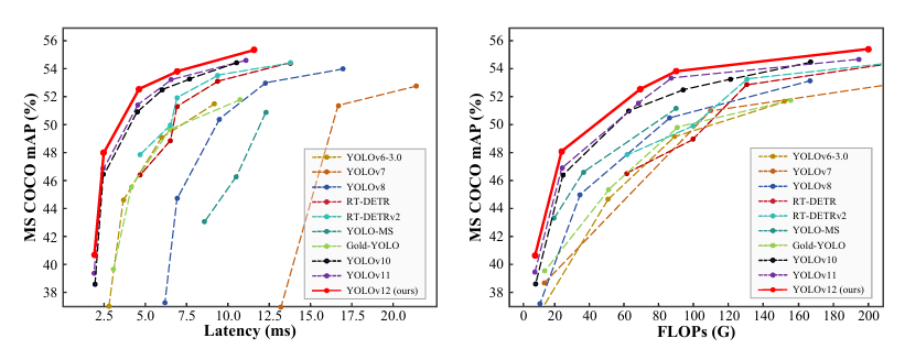
All new models, like YOLO or others, almost always report their performance as an mAP score on a standard dataset like COCO.

IoU for Image Segmentation (Mean IoU)

The IoU is also a crucial metric in image segmentation, used to measure the overlap between two shapes.

Image segmentation involves dividing an image into smaller regions where each part has similar features or qualities. 

Pro tip: Read about Instance Segmentation and Semantic Segmentation.

The segmentation model's output is a "mask," which is a set of pixels predicted to belong to a certain object. The ground truth is also a mask, and we compare these two masks to evaluate the model's prediction.

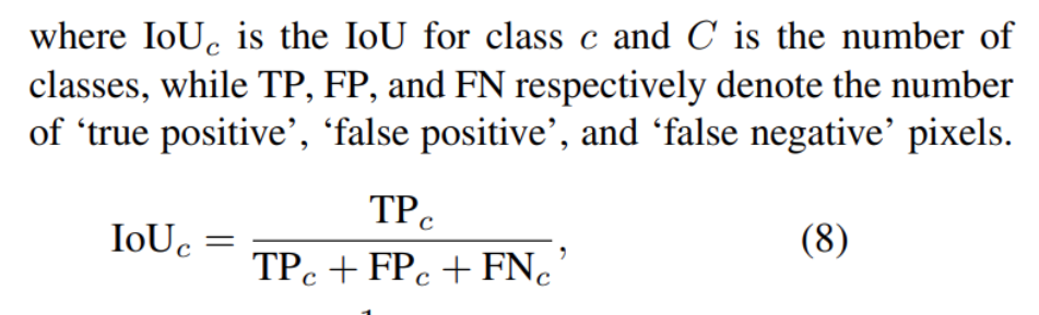
The IoU formula remains the same, but we apply it at the pixel level.

This is equivalent to calculating TP / (TP + FP + FN), where:

• TP (True Positive): Pixels correctly classified as the object.
• FP (False Positive): Pixels labeled as "object" but are actually background.
• FN (False Negative): Pixels that are part of the object but the model missed.

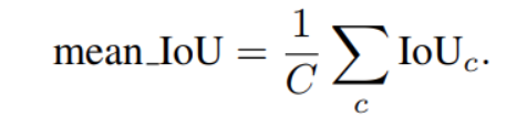
Similar to object detection, segmentation tasks often involve multiple classes, and we calculate IoU for each class separately. Then take the mean Intersection over Union (mIoU), which is the average of these individual IoU scores. 

Beyond IoU: Improved Metrics and Loss Functions

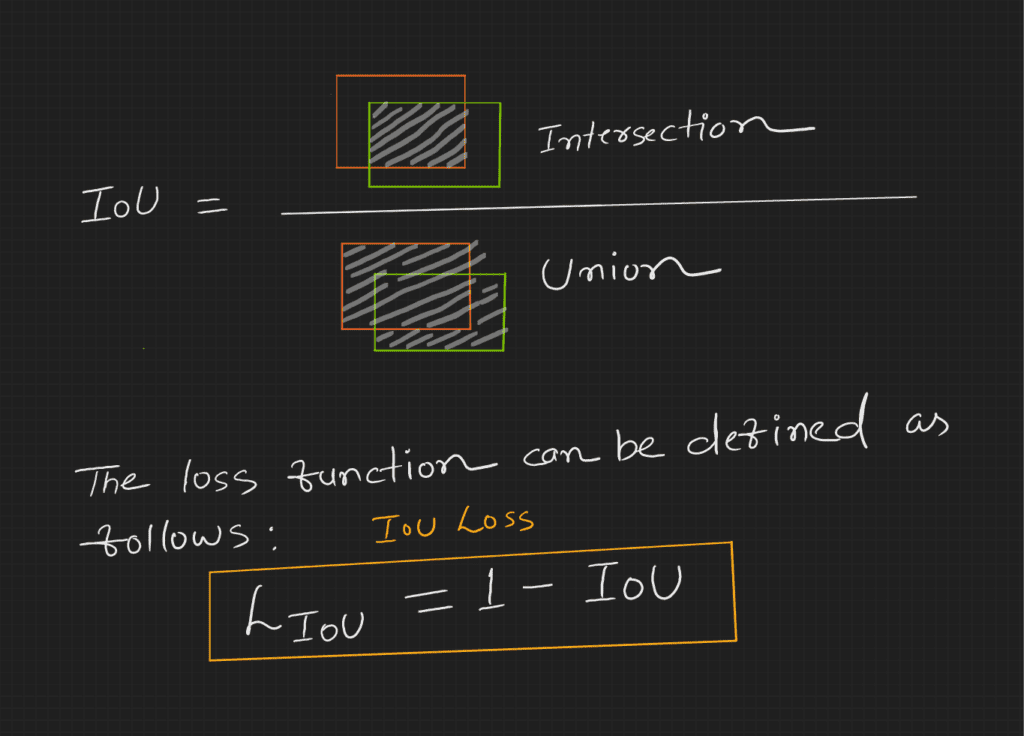
Although IoU is a great evaluation metric, it has some drawbacks when used as a loss function to train a neural network. 

A loss function's role is to show the model how wrong its prediction is and guide it toward a better one.

‍

Here is why to go beyond IoU:

• Zero IoU Problem: When there is no overlap between the ground truth and prediction boxes. In such cases, the IoU is zero, resulting in a zero gradient that prevents optimization and makes it ineffective early in training when predictions likely have no overlap with ground truth.
• Bias Toward Larger Overlaps: IoU weights all errors equally. Sometimes, we might want a metric that also considers how far off a prediction is, even when it doesn't overlap.
  

To address these shortcomings of the standard IoU, researchers introduced Generalized Intersection over Union (GIoU). It improves IoU by using the smallest convex object C that encloses both bounding boxes (A and B). 

Here is the pseudocode for calculating the GIoU:

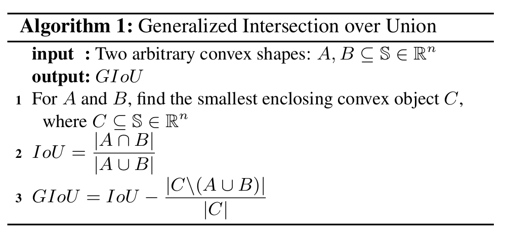
Then the GIoU loss will be calculated as:

Now, even when IoU is zero (no overlap), GIoU is not zero. It becomes a negative value that gets closer to 0 as the predicted box moves closer to the ground truth. It provides the needed gradient for the model to learn and solves the zero IoU problem.

The pseudocode for calculating the bounding box losses:

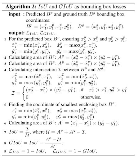
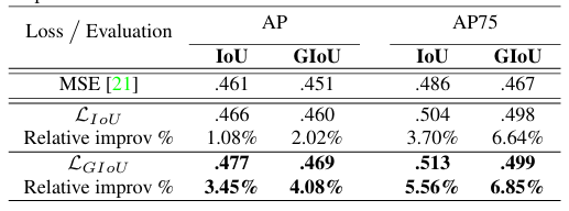
GIoU loss outperforms IoU and MSE loss functions, which result in considerable performance gains in object detection models like YOLOv3.

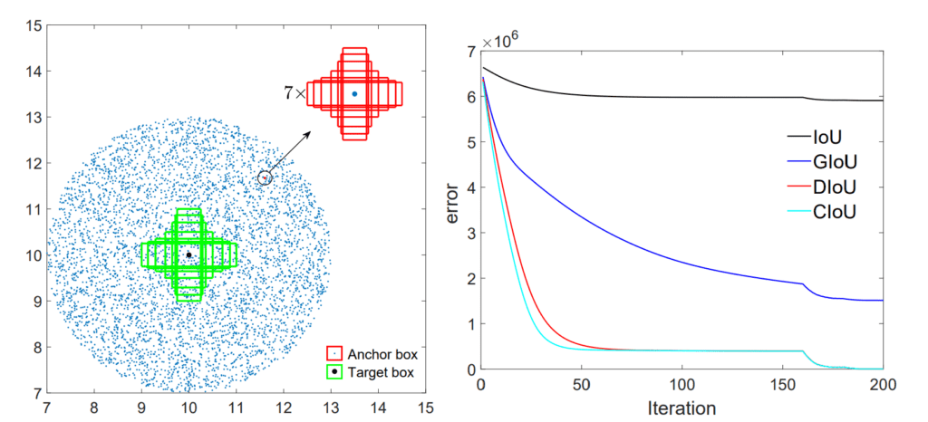
After GIoU, other researchers introduced DIoU (Distance-IoU) and CIoU (Complete-IoU) to improve the convergence even faster and more stably.

DIoU enhances bounding box regression by directly minimizing the normalized distance between the centers of the predicted and ground truth boxes. It makes the loss less dependent on box orientation. 

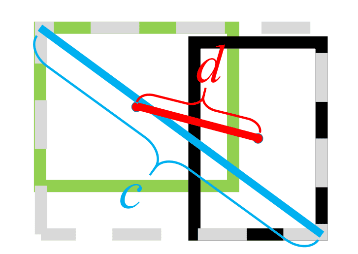
The equation for DIoU loss is:

CIoU extends DIoU by also considering differences in aspect ratio between the boxes. It helps ensure that the predicted box has a similar shape (width-to-height ratio) as the ground truth box.

‍

The CIoU loss function is:

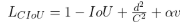
where,

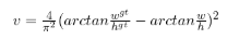
Alpha is a trade-off parameter (function of IoU) and is defined as:

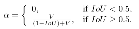
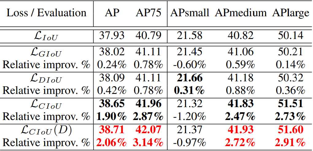
Both DIoU and CIoU show much faster convergence than IoU and GIoU, reaching lower regression errors.

Here is the comparison summary table:

‍

IoU in Practice: Tips, Tricks, and Active Learning Applications

Here are some tips to improve the IoU when building an object detector or segmentation models: 

• Choose Right IoU Threshold: The ideal IoU threshold varies by application, with higher values for high-precision tasks like autonomous driving and possibly lower for cases with small or ambiguous objects. The detection model (Dynamic R-CNN) reports a +5.5% gain in AP at high IoU values.

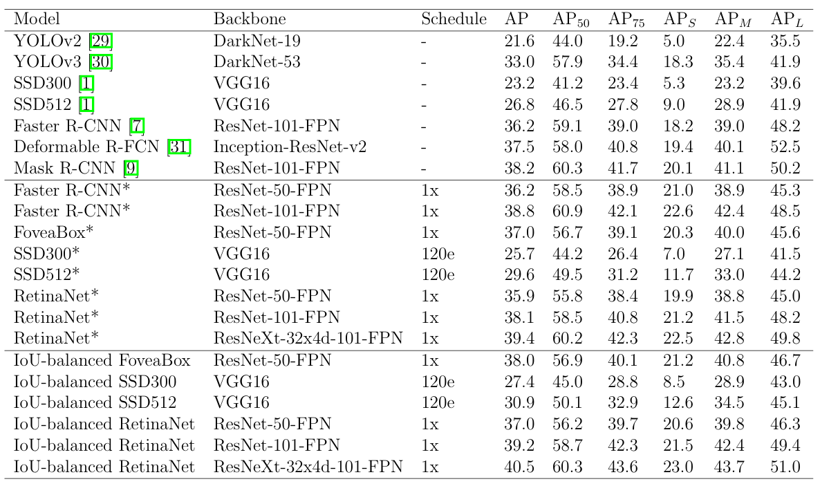
• Improve Models with IoU-Based Loss Functions: Using IoU-balanced or CIoU/DIoU loss increases overall localization precision. For instance, the popular single-stage detectors improve AP75 by up to +2.4%, and AP by up to +1.7%.

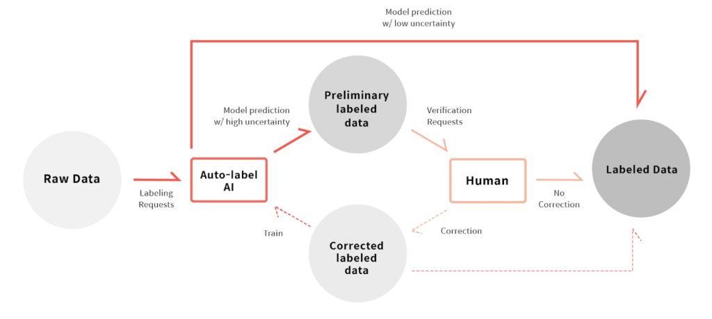
• IoU in Active Learning: Active learning is about selecting the most informative data points to label next, to improve a model efficiently. IoU can be part of the criteria to identify uncertain or problematic predictions:
  
  • Localization Uncertainty: One approach is to look at prediction consistency under perturbations or between model versions. For example, an active learning strategy might compare two similar models' IoU of predicted boxes for the same object.
  • Detection vs Proposal Mismatch: Another strategy looks at the region proposals vs final detections. If a region proposal had a high score but a low final detection IoU or uncertain classification, these could signal edge cases.
  • Diversity and IoU: Active learning also tries to select diverse samples, not just the ones the model is most confused about. IoU can help cluster or distinguish detections.

• Documentation and Source Code: If you’re implementing IoU, many resources are available. Libraries like torchvision have ops.box_iou for pairwise IoU calculation between two sets of boxes. For segmentation IoU, you can use numpy to sum confusion matrices or use sklearn.metrics.jaccard_score for binary masks.

How Lightly AI Improves IoU in Computer Vision Models

Getting high IoU scores in object detection and segmentation starts with training on data that prepares the model for your specific use case.

Public datasets like COCO and ImageNet are useful, but they often lack the unique features of specific industrial or real-world domains. LightlyTrain addresses this by using self-supervised learning. It lets you use your own unlabeled data (images or videos) to build stronger models. 

Instead of starting with generic ImageNet weights, LightlyTrain adapts your model to the specific details of your domain before you begin the fine-tuning with labeled data.

Pretraining on your unlabeled data helps the model learn relevant features, so when you fine-tune on a smaller, curated dataset (like one selected by LightlyOne), it learns faster and more effectively. This results in improved localization accuracy and, as a result, higher IoU scores.

• LightlyTrain GitHub: https://github.com/lightly-ai/lightly-train
• LightlyTrain Documentation: https://docs.lightly.ai/train/stable/index.html

Conclusion

Intersection over Union (IoU) is a key metric that brings clarity to computer vision evaluation, when used with other metrics like mAP. It gives one score that compares the box the model predicts to the true box to see how close they are.

Knowing about IoU helps you better diagnose localization errors and make smarter training choices, from setting evaluation thresholds to using advanced loss functions. With the right tools and data curation, achieving high IoU scores becomes easier and faster.