‍

Contrastive Learning has gained significant traction in recent years, especially in self-supervised and deep learning research. Its ability to learn meaningful representations from unlabeled data has made it a core technique in modern machine learning pipelines. 

The objective is to align or group positive samples together within the latent space and separate or push away the negative samples.

In this article we’ll explore:

1. What is Contrastive Learning?
2. How does Contrastive Learning work?
3. Contrastive Learning - Use Cases (Learning Embeddings)
4. Supervised vs. Self-Supervised Contrastive Learning
5. Contrastive Learning in Computer Vision
6. Contrastive Learning Methods and Frameworks
7. Benefits and Challenges

Contrastive Learning relies heavily on unlabeled data and domain relevance. With LightlyTrain, you can automatically pretrain your models using your own unlabeled images - no manual annotations needed - then fine-tune for tasks like detection or segmentation. Try it out.

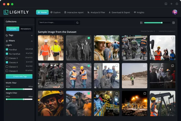
What is Contrastive Learning?

Various families of Self-Supervised Learning methods have emerged in the past few years. One of the most dominant families is Contrastive Learning. Bromley et al. first introduced the idea of Contrastive Learning in 1993, along with the “Siamese” network architecture, in “Signature Verification using a Siamese Time Delay Neural Network” (NeurIPS 1993). Contrastive Learning has significantly impacted almost all forms of modern-day deep Learning, such as Unsupervised, Semi-/Self-Supervised, and fully Supervised Learning.

The core objective is simple: similar things should stay close while different things should be far apart. Contrastive Learning is often employed as a loss function during training. Let’s look at how different methods define contrastive losses.

You can also check out this video for an introduction to Contrastive Learning. 

How does Contrastive Learning work?

In practice, Contrastive Learning often performs best when used in a Self-Supervised manner. 

But how does one do this without labels? 

This is done by creating multiple variants of a single image using a set of known semantic-preserving transformations (data augmentations). All the variants of a given sample become positive, and all others become negative.

Wu et al., in their CVPR 2018 paper titled “Unsupervised Feature Learning via Non-Parametric Instance Discrimination,” provided the first framework that formulated feature learning as a non-parametric classification problem at the instance level and used noise contrastive estimation to tackle the computational challenges imposed by a large number of instance classes.

The question behind the paper was: “Can we learn good feature representations that capture apparent similarity among instances, instead of classes, by merely asking the feature to be discriminative of individual instances?” They used a simple CNN backbone to encode each image into a vector representation, which, after some minor pre-processing (projecting into a lower dimension space and taking its L2 norm), is used to train a classifier to distinguish between individual instance classes.

Weinberger et al.(2009) introduced the Deep Metric Learning paradigm, in which a loss function is broken down into two terms: one that pulls target neighbours closer together and another that pushes differently labelled examples further apart.

‍The “pull” function penalizes large distances between each input and its target neighbours, while the “push” function penalizes small distances between differently labeled examples.

Later works, such as Schroff et al. (2015), introduced the triplet loss, adding a third term as an anchor. This anchor term belonged to the same class as the positive input and differed from the negative input. 

Thus, a model was trained during training to minimize the distance between the anchor term and the positive sample and increase the distance between the anchor term and the negative sample.

NOTE: Over the years, choosing the negative sample proved vital and led to other follow-up work that showcased various ways to select good negative samples (hard negative mining).

Contrastive Learning -  Use Cases  (Learning Embeddings)

An embedding space is a high-dimensional mathematical space where data points are represented as vectors known as embeddings. 

Unlike raw data representations (such as pixel values for images or characters for text), embedding spaces capture meaningful semantic relationships between data points. 

For example, an image model such as ResNet can convert images into embeddings. Converting an image dataset to an embedding space could reveal information about the similarity of various classes. 

So how does one train such a model?

Learning embeddings from a given data distribution arises naturally during contrastive learning. By training a model using “positive” and “negative” pairs using a given distance helps the model understand how “close” or “far apart” two points are in an embedding space. 

Embedding spaces’ have become increasingly important with the rise of dataset sizes. They compress high-dimensional raw data into more manageable representations while preserving essential relationships. Thus one can harness insights about the underlying data distribution by drawing inferences from a lower dimensional (therefore much more accessible) embedding space rather than using the entire raw dataset. 

Embedding Spaces act as a bridge between raw data and meaningful semantic understanding.

While most vision models jointly train an image feature extractor and a linear classifier to predict some label, CLIP (Radford et al., 2021) trains an image encoder and a text encoder to predict the correct pairings of a batch of (image, text) training examples.

Thus, the model learns a multi-modal embedding space by jointly training an image encoder and text encoder to maximize the cosine similarity of the image and text embeddings of the real pairs while minimizing the cosine similarity of the embeddings of the incorrect pairings.

CLIP was a foundational work in the domain of learning multimodal embeddings since it provided a simple scalable framework for learning robust visual features from a text-image dataset. Girdhar et al. (2023) took this approach one step further and proposed an approach to learn a joint embedding space across six different modalities (images, text, audio, depth, thermal, and IMU) in IMAGEBIND: One Embedding Space To Bind Them All.

The authors aim to learn a single joint embedding space for all modalities by binding them with images. Moreover, they align each modality’s embedding to image embeddings. 

Supervised vs. Self-Supervised Contrastive Learning

Now let’s take a quick look at the differences between Supervised vs. Self-Supervised Contrastive Learning.

Self-Supervised Contrastive Learning

In the purely self-supervised scenario, no class labels are used at all instead augmentations/masking is used to provide some supervisory signal during training. This enables learning from raw data and is therefore incredibly valuable in domains where data annotation is expensive such as medical imaging or at scales where manual data annotation is no longer feasible such as in language modelling.

Early successes in this paradigm in computer vision (like CPC, SimCLR, MoCo) demonstrated that unsupervised representation learning with contrastive objectives can rival supervised learning. For example, MoCo’s unsupervised ResNet50 features, when evaluated under the standard linear classification protocol, were on par with a fully supervised ResNet50 on ImageNet​.

‍‍Self-Supervised Learning is the cornerstone of the modern era of LLMs which leverage the vast unlabelled law corpora of text available on the internet. By doing next token prediction and text masking, we no longer need to annotate/categorise text samples.

Supervised Contrastive Learning

But what if we do have access to some supervised labels? Can we still use Contrastive Learning? 

Yes, Contrastive Learning principles can be applied when labels are available too – not just as a pretext task but to directly supervise representation learning.

Supervised Contrastive Learning (SupCon) (Khosla et al. 2020) extends the self-supervised contrastive loss by using labeled information along with the standard objective function. Like in the triplet loss as explained earlier, an anchor and other sample of the same class (since we have access to labels) form the positives samples, while samples of different classes form negatives​. 

This approach was found to outperform the standard cross-entropy loss in image classification, especially when combined with fine-tuning.

Supervised contrastive training tends to produce more robust representations; it has been noted to improve model robustness to data corruptions and hyperparameter settings​. 

This can be seen as a way to further improve the underlying structure of the embedding space. Not only is a model trained for an end task but we also end up enforcing a certain geometric structure on the feature space (best of both worlds: discriminative power of supervised labels and a robust feature space encouraged by contrastive objectives).

Semi-Supervised and Combined Approaches

Contrastive learning also plays a role in semi-supervised learning. 

A common strategy is to first train a model on unlabeled data using self-supervised contrastive learning objective and then fine-tune on the small labeled set. 

This has been shown to yield better performance than training on the labeled set alone. One possible reasoning behind this can be that the model starts off with a much better initialisation. 

While using standard initialization methods lead to stable training, starting off with a model that was pretrained on contrastive learning  provides a much better starting point. For example, SimCLR v2 showed that after unsupervised pretraining using a contrastive learning objective, finetuning on just 1% of ImageNet labels can give substantially higher accuracy than using that 1% data from scratch​.

Most modern multimodal methods use a combination of self-supervised contrastive learning as a way to pretrain models and then fine-tune multiple variants for specific tasks.

For example, Flamingo is a multimodal model that bridges vision and language understanding by using large language models (LLMs) to process and generate text while also understanding images. 

The key innovation behind Flamingo was to use a Perceiver Resampler, which allows a pretrained LLM to incorporate visual data without extensive retraining. Instead of modifying the LLM directly, Flamingo processes image representations from a frozen vision encoder (such as a Vision Transformer or a CNN) and maps them into a format that the language model can interpret. Flamingo was trained using a combination of contrastive learning and causal language modelling.

Contrastive Learning in Computer Vision

So, how do we leverage Contrastive Learning in the computer vision field? Let’s take a look.

Unsupervised Visual Representation Learning

Pretraining techniques for computer vision have evolved significantly over the years with the advent of self supervised contrastive-learning. For instance, it is used by techniques like SimCLR and MoCo to learn image representations by grouping “similar” items together while pushing different items away from each other. These features learnt by such methods are “general” i.e. they can be used to finetune models to a number of downstream tasks. 

Another common approach for visual representation learning is Masked Image Modelling used for training large vision models wherein random parts of images are masked and the model is trained to predict or fill in the missing parts. 

This technique when used in conjunction with scalable architectures like Vision Transformers and methods like Knowledge Distillation lead to extremely capable models.

The MoCo paper demonstrated that contrastively learned features can even outperform supervised features when transferred to image detection tasks. Moreover, DINO suggested that features learnt using Self-Supervised Learning automatically learn features for segmentation without being explicitly trained. 

This suggests the contrastive process uncovers features that are more universally useful.

Contrastive Learning Applications in Computer Vision

Beyond image classification benchmarks, contrastive learning has been applied to a range of computer vision problems. 

For example, in the domain of medical imaging, Multi-Instance Contrastive Learning (MICLe) by Azizi et al. (2021) proposes using contrastive learning for multiple images of the same underlying pathology per patient case. 

Given multiple images from a particular patient, positive pairs are generated for contrastive learning by using two crops from different images, such as from different viewing angles. This enables learning representations that are robust to a change of viewpoint. 

Yang et al. (ICLR 2022), in their paper "Towards Better Understanding and Better Generalisation of Low-shot Classification in Histology Images with Contrastive Learning", introduce Latent Augmentation to better aid few-shot classification in WSIs. They use contrastive learning methods to learn a meaningful encoder in the pretraining stage and their Latent Augmentation strategy to "inherit knowledge" from the training dataset by "transferring semantic variants" in the latent space.Even in reinforcement learning, contrastive learning can help learn state representations from pixels by predicting which future state corresponds to a current state (a form of temporal contrastive learning).

Contrastive Learning Methods and Frameworks

Over the past few years, a variety of contrastive learning frameworks have been proposed, each introducing new ideas to improve performance or efficiency. 

Below is an overview of some seminal methods.

1. SimCLR (A Simple Framework for Contrastive Learning of Visual Representations, 2020)

Chen et al. (2020) proposed the most fundamental framework for using Contrastive Learning for images in their paper “A Simple Framework for Contrastive Learning of Visual Representations”. SimCLR learns representations by maximizing agreement between differently augmented views of the same data example via a contrastive loss in the latent space.

This framework had some simple components:

• Given an input image, two “views” are generated using augmentations sampled from known semantic-preserving transformations, such as random colour distortions or random Gaussian blur.
• These views are then encoded into vectors using an encoder model. A typical choice for the encoder model is the backbone of a pretrained image classification model.
• A small projection head then maps these representations into a latent space, where the contrastive loss is finally applied.

A random minibatch is sampled, and then augmented examples are generated. After generating augmented views for N samples, we’ll get 2N data points (2 views of each sample). Note that we don’t explicitly search for hard negative samples. Instead, given a positive pair, all other 2(N-1) samples are treated as negative pairs.

2. Barlow Twins (2021)

Along the same lines, Zbontar et al. (2021) proposed a similar framework. Still, instead of a similarity-based contrastive loss, they enforced the cross-correlation matrix between the features from augmented views to be close to the identity.

For a given pair of views, the loss function employed by Barlow Twins is as follows:

‍

The first term here minimizes the invariance by equating the diagonal elements of the cross-correlation matrix to 1, thereby making the embedding invariant to the distortions applied. In contrast, the second term reduces the redundancy by trying to equate the off-diagonal elements of the cross-correlation matrix to 0, thereby de-correlating the various vector components of the embedding.

3. VICReg (Variance-Invariance-Covariance Regularization, 2021)

The VICReg framework by Bardes et al. (2022) goes one step further with the framework introduced by SimCLR and Barlow Twins for training joint embedding architectures based on preserving the information content of the embeddings.

The loss function used in VICReg combines three terms: an invariance term that minimizes the mean-squared distance between the embedding vectors, a variance term that forces the embedding vectors of samples within a batch to be different, and a covariance term that de-correlates the variables of each embedding and prevents an informational collapse in which the variables would vary together or be highly correlated. The final loss is a weighted average of the invariance, variance and covariance terms.

Others: There are many other notable methods: PIRL (prior to SimCLR, proposed using jigsaw patches as positive pairs), SwAV (Swapping Assignments between Views, which performs contrastive learning by clustering assignments instead of instance pairs) and CLIP.

‍

Benefits and Challenges of Contrastive Learning

As mentioned so far, the use of contrastive learning has proved powerful for pretraining since it’s extremely effective at extracting meaningful representations from raw data. These learnt embeddings tend to be more robust and information rich when compared to the features learnt from standard supervised learning. 

Thus, contrastive learning can be used during pretraining to train models with a good general understanding (even with multimodal datasets) and then be further fine tuned on a number of downstream tasks. It has been empirically shown that using models pretrained using contrastive learning perform better when evaluated compared to random initialisation.

Challenges and Limitations

Despite its success, contrastive learning comes with many challenges. A key issue is the requirement of either large batch sizes or memory mechanisms to provide many negative examples – this can make training expensive in terms of GPU memory or training time. Methods like MoCo alleviated this, but the fundamental need for a variety of negative samples remains (unless one uses the BYOL/SimSiam approach).

Another challenge is choosing effective data augmentations: remember, the model will only be invariant to what you augment. If your augmentations are too weak, the model might focus on superficial differences; if they are too strong (or not carefully chosen), the model might sometimes be forced to treat very dissimilar inputs as “same,” therefore hurting the overall learning process. 

Data augmentation can however also be viewed from a positive lens since if chosen appropriately then can be used to alleviate bias in the dataset.

Hard Negative Mining

As alluded to, not all negative samples are equal. There is ongoing research into mining difficult negative samples that yield more training signal. 

Hard negatives can prevent the model from getting complacent by only seeing obviously different negatives. However, identifying which negatives are “hard” without labels is tricky, and using false negatives (actually similar pairs treated as negative) could confuse training. 

It has been recently shown however that by using high batch sizes one can alleviate the need of finding negative samples, but that of course comes with the constraint of having access to large amounts of compute.

Conclusion

Contrastive learning is both one of the key pillars of representation learning and a key framework in self supervised learning. In contrastive learning, multiple views are generated from a given sample and then "contrasted" with views from other samples. The various views from a sample are regarded as positives and those from other samples are negatives. 

By learning to recognize which pairs are related and which are not, the model develops some form of understanding of the underlying structure of the data (a stronger geometric constraint). 

The success of Contrastive Learning has led to significant improvements in the quality of learned representations, often rivalling or surpassing those obtained through traditional supervised learning methods.