Demystifying the Confusion Matrix: A Short Guide
Table of contents
Share blog post


A confusion matrix is a table that compares predicted vs. actual labels, detailing true positives, false positives, false negatives, and true negatives. It helps evaluate classification accuracy, diagnose errors, and compute metrics like precision and recall.
Share blog post
Below, you can find a quick summary of key points about the confusion matrix.
What is a confusion matrix?
A confusion matrix is a table that compares a machine learning model's predicted class labels with the actual labels. It shows counts of true positives, false negatives, false positives, and true negatives to give detailed insights into model performance.
Why use a confusion matrix in machine learning?
It reveals where a classification model makes mistakes. Engineers gain specific insights into false positives and false negatives to improve the model’s generalization performance.
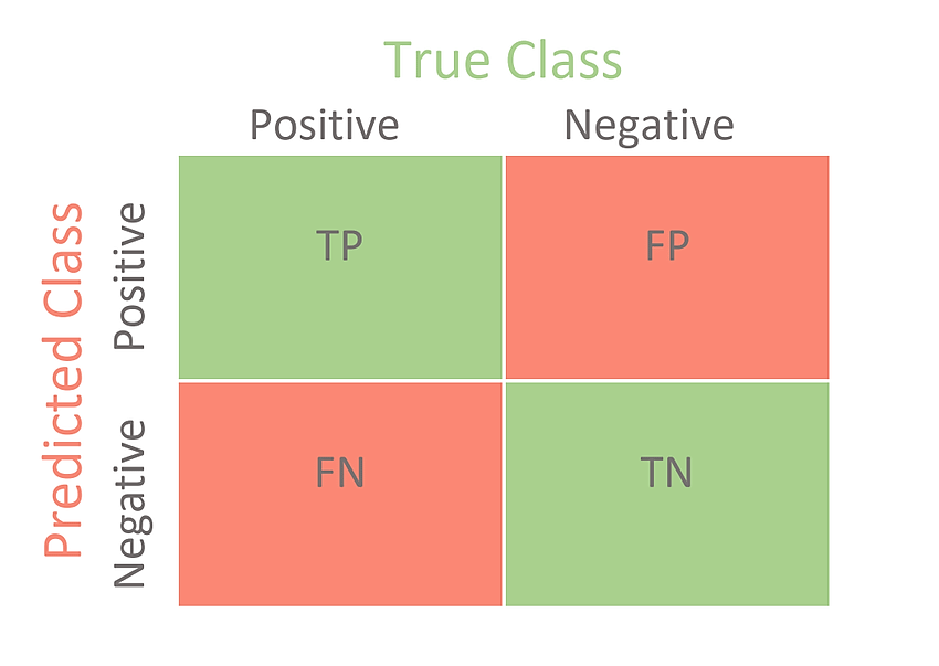
What do terms like True Positive, False Negative, etc, mean?
These terms refer to the four outcomes in the confusion matrix:
- True Positives (TP) are the correct positive predictions
- False Positives (FP) are the incorrect positive predictions
- False Negatives (FN) are the missed positive cases
- True Negatives (TN) are the correct negative predictions
How do you calculate precision and recall from a confusion matrix?
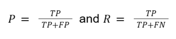
Precision (P) measures the correct predicted positives or the true positive rate, and recall (R) measures the true instances that are correctly identified. They are calculated using:
Can confusion matrices handle multi class classification?
Yes. Multi-class confusion matrices are NxN tables where rows represent actual classes and columns represent predicted classes. This helps evaluate model performance in complex scenarios like image classification.
Introduction
Accuracy alone can be misleading in machine learning (ML). A model may show strong overall performance but still fail to detect rare yet critical cases.
To properly evaluate a model’s performance, you need tools that go deeper and highlight both strengths and weaknesses.
This is where the confusion matrix becomes essential.
This guide covers all you need to understand about confusion matrices, evaluation metrics, and how to fit them effectively into ML workflows.
We will explore the following:
- What is a confusion matrix
- Interpreting the confusion matrix
- Key evaluation metrics derived from the confusion matrix
- Multi-class confusion matrices
- Why confusion matrices matter for model performance evaluation
- Confusion matrix in practice
- Tips, best practices, and challenges
- How Lightly AI supports confusion matrix analysis and data quality
Improving your confusion matrix results starts with improving your data. At Lightly, we help you train models that make fewer false positives and false negatives by focusing on data quality and relevance:
- LightlyOne: Curate balanced, representative datasets to ensure your model learns from the most informative samples.
- LightlyTrain: Pretrain and fine-tune models on curated data for better generalization and more reliable evaluation metrics.
Together, they help you build models that perform consistently across classes—and make your confusion matrices truly meaningful.
See Lightly in Action
Curate and label data, fine-tune foundation models — all in one platform.
Book a Demo
What is a Confusion Matrix?
A confusion matrix, sometimes called an error matrix, is a tool for evaluating the performance of a classification model or algorithm. It compares predicted labels with ground truth labels using test data.
It shows counts of true positives, false negatives, false positives, and true negatives for detailed insights. ML engineers can get a clear breakdown of the model’s performance by listing how often each prediction matches the real value.
Binary Confusion Matrix
In a binary classification problem, the confusion matrix is a 2×2 table that summarizes prediction results. It organizes the predictions into four categories:
These counts provide the basis for calculating all important evaluation metrics. It also highlights the types of mistakes the model makes, which can indicate areas where it needs improvement.
Interpreting the Confusion Matrix
A confusion matrix shows where a classification model performs well and where it struggles. True positives and true negatives represent correct classifications, while false positives and false negatives show incorrect predictions.
Simultaneously, the error matrix shows which types of errors are most common. In multi-class classification models, confusion matrices also show which actual classes are most often confused with which predicted classes.
To understand how a confusion matrix is interpreted, consider an example of a spam classification model that labels emails as ‘spam’ or ‘not spam’:
- TP: Emails correctly flagged as spam
- FP: Legitimate emails wrongly flagged as spam
- FN: Spam emails that slipped through as normal
- TN: Normal emails correctly passed
Suppose the model was tested on 100 emails. 50 were actually spam, and 50 were legitimate. It correctly labeled 45 of the actual positive instances, but it missed 5 of them.
Among the legitimate emails, it accurately marked 47 as noise (not spam), but mistakenly flagged 3 as spam, where the true label was not spam
The resulting example confusion matrix shows:
To calculate accuracy:
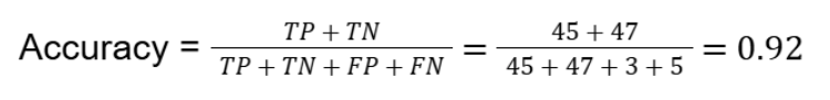
Instead of relying only on a 92% high accuracy, the matrix reveals the trade-off between false alarms and missed spam in the model. This insight guides targeted adjustments such as recalibrating classification thresholds or increasing the training data set for difficult cases.
Pro tip: To better understand how models classify images before they even reach evaluation, check out our Guide to Image Classification. It explains model architectures, techniques, and best practices that complement confusion matrix analysis.
Key Evaluation Metrics Derived from the Confusion Matrix
The metrics derived from the confusion matrix highlight both the strengths and weaknesses of your classification model. This overcomes the limitation of accuracy as a metric, which often favors the majority class, making it unsuitable for imbalanced datasets.
The matrix helps you calculate Precision (P) and Recall (R). Precision becomes especially important when false positives are costly. For example, in fraud detection, wrongly flagging legitimate transactions can frustrate customers.
In contrast, Recall (R) is critical when missing positives are risky. For example, in disease diagnosis, missing an illness can put patients' lives at risk. Whereas the F1 Score (f-score) balances both precision and recall aspects to optimize overall classification quality.
| Metric | Formula | Interpretation |
|---|---|---|
| Accuracy | 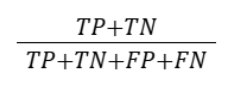 |
Proportion of correct predictions overall |
| Precision | 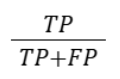 |
How many positive predictions are positive (e.g., spam filters) |
| Recall | 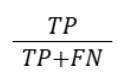 |
How many actual positive instances were found (e.g., medical tests) |
| F1 Score |  |
Balances precision and recall (harmonic mean); useful for skewed data |
| Specificity | 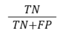 |
Correct negatives among negatives |
| False Positive Rate | 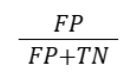 |
Portion of negatives wrongly classified as positive |
| False Negative Rate | 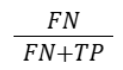 |
Portion of positives missed by the model |
Multi-Class Confusion Matrices
For problems with multiple classes, the confusion matrix extends to an N × N grid, where N is the number of classes.
For example, in a 3-class image classification, the matrix highlights which pairs of classes (i.e., cats, dogs, and rabbits) the model confuses. This is similar to a binary matrix extended to multiple classes.
For such cases,
- Each row corresponds to the actual class
- Each column represents the predicted class
- Diagonal cells show counts of correct predictions per class
- Off-diagonal cells show misclassifications or mistakes between classes

Here is an example confusion matrix of a 3-class image classification task for animal species. A computer vision model is trained to classify cats, dogs, and rabbits.
After testing on 300 images (100 per class), the confusion matrix looks like this:
Here, the model confuses rabbits and dogs more often than other pairs (i.e., cats). This insight guides data collection strategies due to similarities in those image features.
Evaluating Multi-Class Models
To evaluate multi-class performance, we often compute the same metrics (precision, recall, F1) for each class individually. This calculation can be done by averaging in several ways, such as:
- Macro-average: Average metric scores for all classes equally
- Micro-average: Aggregate counts across all classes to calculate metrics globally
- Weighted average: Average metrics weighted by the number of samples per class
Why Confusion Matrices Matter for Model Performance Evaluation
With imbalanced datasets, high accuracy alone can be misleading because it can hide poor performance on rare but important classes. A multi-class confusion matrix shows the true positives, false positives, and false negatives. This makes the error distribution visible for each class.
Using confusion matrices allows AI builders and teams to spot frequent mistakes and improve multi-class classification models. This also helps select better evaluation metrics, such as F1 score or ROC curves.
Confusion matrices can reveal if certain classes are consistently misclassified or ignored. This can indicate bias in the model. That is why it is crucial to ensure ethical artificial intelligence (AI) deployment to help fine-tune thresholds.
When working with classification models that produce probabilities, thresholds determine whether an instance is labeled as positive or negative. Adjusting thresholds changes the trade-off between false positives and false negatives.
For example, raising the threshold reduces false positives but increases false negatives.
Additionally, the receiver operating characteristic (ROC) curve plots the true positive rate against the false positive rate at various threshold settings. It helps choose the threshold that best balances sensitivity and specificity.
The ROC analysis complements the confusion matrix insights by visualizing classifier performance across different thresholds.
Confusion matrices support targeted improvements. Engineers can gather more samples for problematic classes, refine features, or retrain models with attention to weak areas. This improves the correct classifications of predicted classes and helps stakeholders understand the model’s performance.
💡Pro Tip: To correctly interpret YOLO detection results beyond mAP, our YOLO Object Detection Explained guide helps connect confusion matrix patterns to common localization and classification errors.
Confusion Matrix in Practice: Applications and Examples
Confusion matrices are commonly applied across various domains to help evaluate and refine classification models. Below, we will discuss several use cases with detailed examples.
Binary Class Medical Diagnosis
In a binary classification problem, the model predicts the patients as positive or negative for detecting the disease. For such cases, mislabeling a small subset as a false negative (missing a disease) can be a seriously fatal error. However, false positives may lead to further testing but are less harmful.
Research on tuberculosis (TB) detection using ResNet50 achieved 91% accuracy, with precision at 80% and recall at 90.9%. Here, high recall indicates the model successfully detects most TB cases, minimizing missed diagnoses.
Slightly lower precision signals that some of the false positives remain. Confusion matrix analysis helps balance these metrics to reduce critical errors and avoid excess unnecessary testing.
Multi-Class Image Classification
Computer vision tasks benefit significantly from confusion matrix analysis.
In a skin cancer study, multi-class confusion matrices showed which types of lesions the model often confused. This helped researchers decide where to collect more data or adjust the model to ensure predicted values are correct.
In another research, the multi-species recognition models showed confusion between wolves and dogs, due to subtle feature similarities. This observation shows model enhancement and data collection strategies in such cases.
Model Monitoring and Drift Detection
High accuracy alone only summarizes overall model performance but misses changes in specific error types. Confusion matrices show detailed shifts in false positives and false negatives that might not immediately impact overall accuracy but indicate model drift.
Spam Filtering
Confusion matrices are essential for tuning spam filters. Too many false positives frustrate users by blocking legitimate emails, whereas false negative exposes spam content. These spam filtering systems often deal with imbalanced datasets where spam emails are rare.
The confusion matrix helps identify whether too many legitimate emails are being wrongly blocked or if spam emails are being missed. Using this insight, ML engineers can adjust the classification model threshold to effectively balance user experience and security.
Active Learning Workflows
In active learning, models flag uncertain or misclassified samples via the confusion matrix feedback. These matrices reveal which classes cause the most confusion, which helps select samples for data annotation.
Focusing on these ‘confused’ cases lets models learn faster with fewer labels. This targeted approach beats the random sampling method, especially when model predictions are uncertain or inconsistent.
Pro tip: Selecting the right annotation tool is crucial when building efficient active learning pipelines. Check out our list of Top 12 Best Data Annotation Tools to explore options that speed up labeling and improve dataset quality.
Using Tools and Libraries
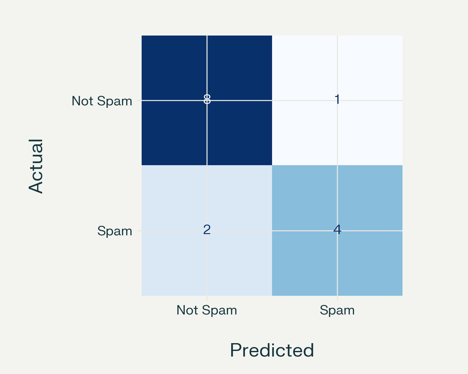
Generating confusion matrices is straightforward with open-source libraries such as scikit-learn. Below is a simple Python example for email spam detection:
import matplotlib.pyplot as plt
from sklearn.metrics import confusion_matrix, ConfusionMatrixDisplay


# Email spam detection results
y_true = [0, 0, 0, 0, 0, 1, 1, 1, 0, 0, 1, 1, 0, 0, 1]  # Actual labels (0: not spam, 1: spam)
y_pred = [0, 1, 0, 0, 0, 1, 0, 1, 0, 0, 1, 1, 0, 0, 0]  # Model predictions


target_names = ['Not Spam', 'Spam']
cm = confusion_matrix(y_true, y_pred)
disp = ConfusionMatrixDisplay(confusion_matrix=cm, display_labels=target_names)


fig, ax = plt.subplots(figsize=(5, 4))
disp.plot(ax=ax, cmap='Blues', colorbar=False)
plt.title('Email Spam Detection - Confusion Matrix')
plt.xlabel('Predicted')
plt.ylabel('Actual')
plt.tight_layout()
plt.savefig('confusion_matrix_example.png')
plt.show()
Output
Using Confusion Matrix: Tips, Best Practices, and Challenges
Using confusion matrices effectively requires careful attention to how they are set up and interpreted.
If not handled correctly, they can lead to wrong conclusions about the performance of your ML models.
Tips and Best Practices
To get the most value from confusion matrix analysis, here are some practical tips and best practices you should consider:
- Always check matrix orientation: Confirm whether your tool sets rows as actual classes and columns as predicted classes, or vice versa. Misinterpretation can lead to wrong conclusions.
- Normalize values for clarity: For easier comparison in imbalance datasets, express true positives, true negatives, false positives, and false negatives as percentages or rates.
- Use alongside other important metrics: Pair confusion matrix analysis with ROC curves, precision-recall curves, and other domain-specific metrics.
- Handle imbalanced datasets deliberately: Use sampling techniques or class-weight adjustments during the training to prevent biased or uncertain models.
- Continuously monitor models: Use visualization tools and track confusion matrices on the production data to detect model drift or changing data distributions.
Challenges
Despite their usefulness, confusion matrices also come with some challenges. These include:
- Sensitive to threshold choice: Confusion matrix results change a lot depending on the threshold you set for classification. If two models use different thresholds, their results can not be fairly compared.
- Ignoring small sample sizes: Metrics from very small datasets may be misleading or unstable. This is because limited data can cause high variance in evaluation results and reduce confidence in the model’s true performance.
- Failing to monitor over time: A model that performed well initially might degrade gradually as new data with different patterns arrives unexpectedly.
- Overlooking context: The cost of false positives vs false negatives varies widely across applications. Understanding your domain is essential to making correct decisions.
How Lightly AI Supports Confusion Matrix Analysis and Data Quality
Lightly AI helps teams turn insights from confusion matrices into real improvements by offering smart, practical tools that support every step of the machine learning pipeline.
LightlyOne
LightlyOne helps select the most valuable data samples for labeling. It targets uncertain or misclassified samples highlighted through confusion matrix analysis.
LightlyOne uses advanced similarity analysis and an active learning cycle to accelerate the improvement of the classification model.
LightlyTrain
Training a model from scratch usually takes a large amount of labeled datasets. LightlyTrain cuts that down by using self-supervised learning to learn patterns from unlabeled data first.
That way, your model starts off with stronger feature representations. This makes it better at telling apart similar classes and reducing the false positives and false negatives you’d otherwise see in a confusion matrix.
LightlyEdge
Models in production often face new data that causes drift. LightlyEdge captures challenging or unusual inputs directly on edge devices, even with limited compute power. These samples can then be fed back into the pipeline.
This helps the model stay stable and reduces the risk of performance drop over time.
Conclusion
A confusion matrix helps machine learning teams identify where a classification model makes accurate predictions and where it fails. It supports tuning thresholds, handling imbalanced datasets, and improving multi-class predictions.
Used with other important metrics, the confusion matrix ensures reliable AI models for applications from medical diagnosis to fraud detection.

Stay ahead in computer vision
Get exclusive insights, tips, and updates from the Lightly.ai team.


.png)
.png)