‍

Training a machine learning (ML) model is only a small part of a project. 

The real challenge is building the entire system around it. You need a reliable way to convert messy raw data into a trained model ready for production. 

This is where the ML data pipeline comes in, managing everything from raw data to the final model. 

In this guide, we'll walk you through each step of building a powerful computer vision pipeline.

Here’s what we cover:

1. What Is a Computer Vision Data Pipeline?
2. Planning and Data Collection 
3. Data Labeling and Annotation 
4. Data Preprocessing and Cleaning
5. Feature Engineering and Representation 
6. Splitting Data: Training, Validation, and Test Sets
7. Model Training: Selecting and Training Your Machine Learning Model
8. Model Evaluation and Validation 
9. Deployment and Monitoring 
10. How to Build Better Computer Vision Data Pipelines with Lightly AI

Most teams struggle to build and manage ML data pipelines, especially the data processing and selection stages. 

At Lightly, we empower teams to fix this problem and improve their machine learning models by using the best data.

• LightlyStudio: It helps you curate and annotate your dataset, identify hard-to-see edge cases, and use active learning to select only the samples that will improve model performance.

• LightlyTrain: Pretrain models on unlabeled data using self-supervised learning. This helps models learn relevant features of your domain before they see a label.

Try both for free and see how they can fit into your machine learning workflow.

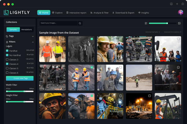
What Is a Computer Vision Data Pipeline? 

A computer vision data pipeline is the end-to-end path that image and video data take in an ML project. 

It starts with data ingestion (images captured or uploaded) and proceeds through the preprocessing, annotation, training, and evaluation steps to final model deployment.

In short, it’s the machine learning pipeline specifically for vision tasks.

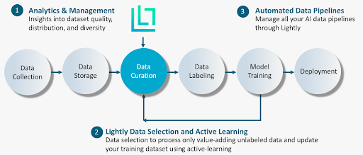
We can think of the ML pipeline workflow as three key stages:

• Data Processing: It's an initial phase that involves collecting, cleaning, labeling, and transforming raw data into a format suitable for training.
• Model Development: It includes choosing the right algorithms (model selection), training, and tuning them. Also, include an evaluation where we thoroughly assess the model's performance.
• Model Deployment: The last step in the ML pipeline, where we are deploying models into a production environment. It makes predictions on new, unseen data, with an ongoing monitoring and feedback loop to maintain performance.

Since data preparation dominates ML, without such a pipeline, engineers and data scientists spend lots of time (roughly 60%) doing manual tasks (renaming files, retraining models from scratch). 

A good pipeline automates these repetitive tasks and ensures reproducibility. It also helps keep things organized with clear folder structures and metadata, so teams don’t overwrite each other’s work. 

Over time, using such pipelines leads to more consistent results and reduces waste of time and resources.

Planning and Data Collection 

Every machine learning project begins with a plan. You cannot build a pipeline without knowing what you're building it for (its purpose). 

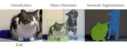
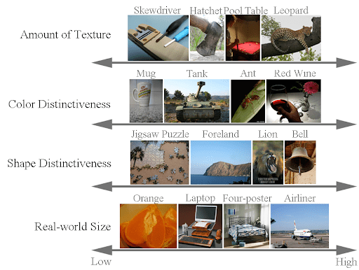
So, first decide what problem you are trying to solve with computer vision (CV task). Are you classifying images, detecting objects, sementing scenes, or something else, like pose estimation or OCR? Knowing the task helps you find what data you will need.

For example, if you're doing object detection, you'll need images with bounding boxes drawn around the objects of interest. If you're classifying images, you only need one label per picture.

Once you know the task, the next step is to identify what kind of images or videos you need (visual data requirements). 

Consider image format (RGB color, infrared, depth), resolution (high-res vs thumbnail), whether they are stills or video frames, diversity needed, and indoor vs outdoor settings. And then, decide how much data is enough to start training the model.

Once you know what you need, you can figure out how to get it. 

Computer vision datasets can come from many places:

• Public Datasets: There are many public datasets that we can use to start with our CV projects. For example, ImageNet (large-scale image classification), COCO (object detection/segmentation), OpenImages, Cityscapes (street scenes), KITTI (autonomous driving), and MNIST. We can save much of our data collection time using these established datasets.

• Web Scraping and APIs: If public datasets do not cover your niche, you can gather images from the web using search engine APIs or image search tools. Tools like Google Images API or Flickr API can help collect large batches.
  
  
• Sensors and Edge Devices: If you have cameras, drones, or embedded devices on-site (in a warehouse, production line, or in the field), you can collect domain-specific data right at the point of capture. To do this, you can use tools such as LightlyEdge.

• Since LightlyEdge SDK can run on the camera itself, it uses embedded model inference to filter and select only the most informative frames in real‐time. Thereby reducing storage, upload, and labeling costs. It also helps you collect some metadata, which can be useful when you perform feature engineering or for future debugging.

• Simulation or Synthetic Data: In some cases, it’s faster to generate synthetic images, especially when real data is scarce or contains many rare or /edge cases. Tools like graphics engines (Unity, Blender) or simulators (CARLA, AirSim) can produce labeled images with perfect ground truth. 

• You can also request Lightly's AI Data Services for high-quality synthetic data tailored to your domain. It combines synthetic data with real data (hybrid approach) and expert human-in-the-loop annotation to build stronger training sets and to cover edge cases.

Pro Tip: You can also check out our list of 5 Best Data Annotation Companies in 2025 [Services & Pricing Comparison].

Data Labeling and Annotation

Once you have raw images, the next step is labeling them according to the task. No matter how advanced the architecture we use, it can only learn from the labels we give it. 

If your labels are noisy or inconsistent, the model’s performance will suffer, and will lead to garbage in, garbage out. Therefore, you need to invest time here to get the annotation right.

Annotation Workflow

You must first decide on an annotation strategy, like who will label the images or videos and how you will manage the workflow.

The options you have are in-house team members (with domain expertise) or crowdsourcing using platforms like Amazon Mechanical Turk, for scale. 

For tooling, you need an annotation platform that supports labeling, dataset management, versioning, class management, export formats, and ideally, data selection.

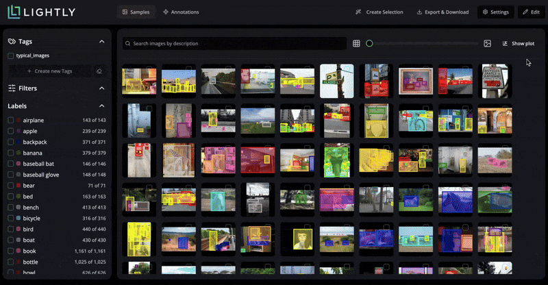
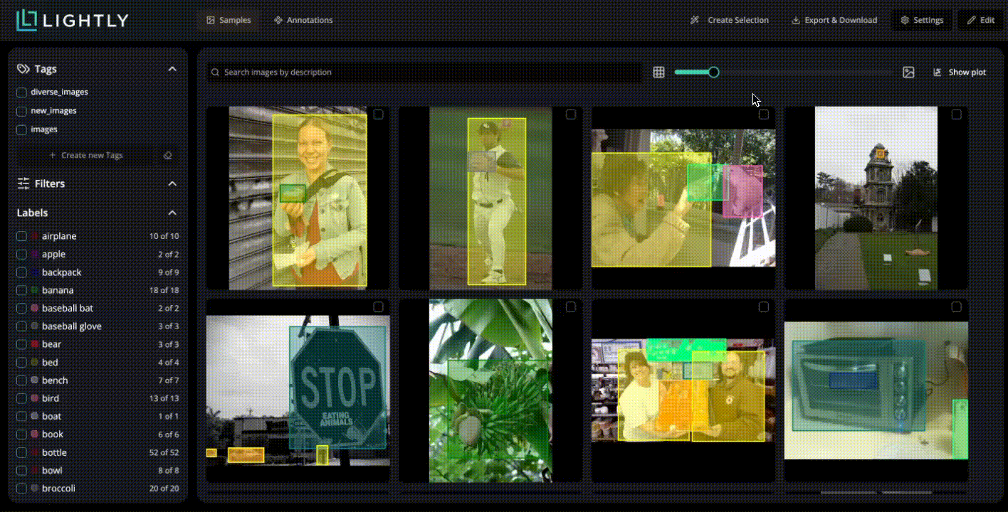
Popular open-source tools include LabelImg, CVAT, and LightlyStudio (unifies annotation with dataset curation).

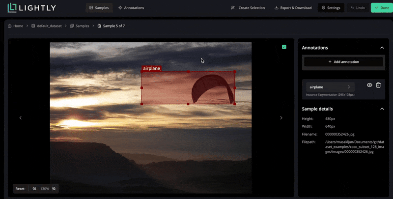
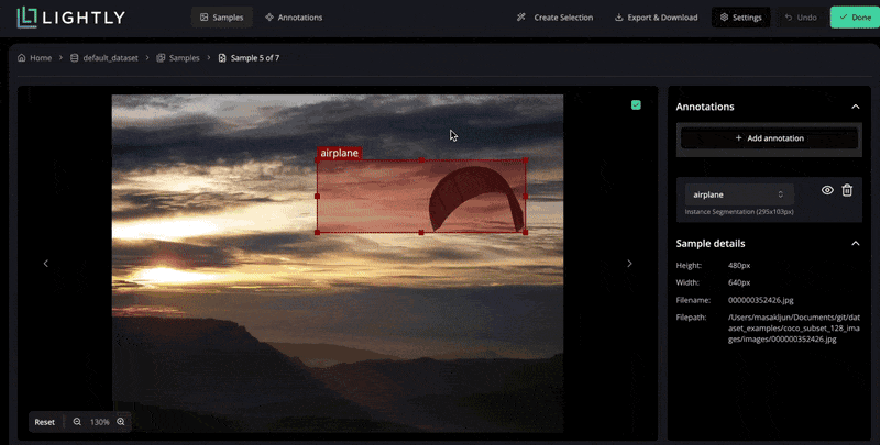
In LightlyStudio, you can upload your images, run through a simple labeling interface, and use embedding-based selection at the same time.

It computes visual embeddings for all images and lets you query or filter them, like show me images containing animals. This way, you prioritize annotation effort on the most relevant samples.

Pro tip: Check out 12 Best Data Annotation Tools for Computer Vision (Free & Paid)

LightlyStudio supports various annotation types, including bounding boxes, segmentation masks, and also helps manage label classes and exporters (COCO or YOLO). 

Quality Control

Annotation quality is critical, since poor labels undermine model performance even before training begins.

Common practices include double-blind annotation (two people label the same image and reconcile differences), consensus voting, or spot audits (review a random sample of labels). 

For example, in object detection, you might catch mislabeled boxes by visual inspection. If possible, implement a review step where a second expert validates a subset of annotations. 

Another approach to ensure quality is by visualizing the embeddings. LightlyStudio helps visualize the dataset structure to locate near-duplicates and spot anomalous samples or groups that may be mislabeled.

Active Learning Loop

Instead of labeling all your data up front, use an active learning approach that lets you label more intelligently. It focuses on annotation effort where it delivers the most value, reducing cost and maximizing performance.

To scale active learning, use tools like LightlyStudio that support this loop with built-in automation and tooling. 

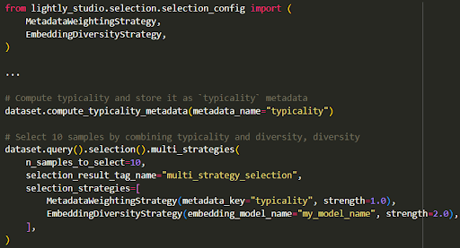
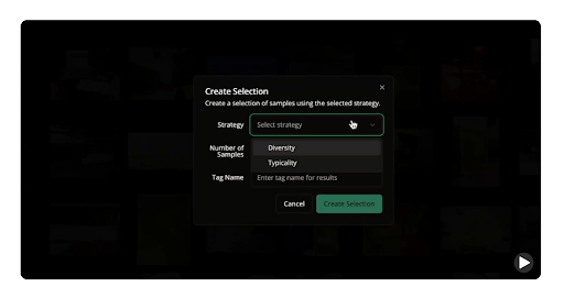
It computes visual embeddings for all samples and supports selection strategies, such as diversity-based and metadata-weighted. Then you can select the most valuable unlabeled data to label using those strategies. 

The LightlyStudio Python SDK facilitates active learning in ML pipelines by enabling scriptable selection logic, sample tagging, and annotation export or import.

LightlyStudio also supports multi-strategy selection. You can combine embedding diversity, metadata weighting, and uncertainty heuristics for more optimal sample selection. Here is how you can do:

Annotation Metadata and Data Imbalance

Just like the data itself, labels should be versioned. Keep track of annotation versions (especially if labels change over time). 

Use tools or naming to record when an annotation batch was created or updated. If the model’s accuracy drops after adding new labels, you need to know what changed.

Also, during the labeling process, it is important to be aware of class imbalance. If one class appears far more frequently than others, the model may become biased. 

Monitoring class distributions during annotation can help identify and mitigate this issue early on.

Data Storage and Version Control

At this point, you have raw and labeled data, so organize it rigorously. Good data management involves establishing a structured system for storage and implementing version control.

Key practices:

• Centralized Data Repository: You should store all data (raw images, annotations, and intermediate files) in a central location (repository) accessible to all team members and pipeline processes. Cloud storage services like AWS S3 or Google Cloud Storage are popular for their scalability and accessibility. Alternatively, network file systems or on-prem object storage can work for large image volumes.

• Folder Structure and Naming Conventions: A clear and consistent folder structure is essential for organization. So, use descriptive folder and file names, as they help anyone new to the project easily understand where to add or find data.

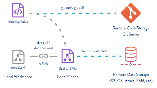
• Dataset Versioning: Use version control systems or data versioning tools to track changes. Tools like DVC (Data Version Control) let you record each version of your dataset (version 1.0 with 5k images, version 1.1 adding 1k more). It works with Git to track large data files without storing them in Git itself. It allows you to check out previous versions of your dataset as needed.

• Folder Structure and Naming Conventions: For large-scale pipelines, a data catalog or metadata management system (MLflow Tracking for datasets) can be used to manage metadata. These tools store information about each dataset, such as its source, creation date, version, and schema.

• Access Control and Intermediate Outputs: The storage system must be configured with proper access controls to ensure data security. Furthermore, a CV pipeline often produces intermediate artifacts like resized images, extracted features, embeddings, augmented datasets, and model checkpoints. These outputs should also be stored systematically, as logging them makes debugging easier (if something goes wrong).

Data Preprocessing and Cleaning 

Data preprocessing is the step where we take unrefined data and organize it into a clean and consistent format so that a model can learn from it effectively. 

Data Cleaning

Raw data is rarely ready for model training, so the first step in cleaning is to correct or discard any faulty data.

It includes removing duplicate images (two identical photos that take up unnecessary space) and deleting corrupt files or unreadable pictures. It also involves filtering out images that are irrelevant (off-topic) or have unusual resolutions.

Moreover, ensure the label consistency and images without labels or with questionable labels should either be correctly labeled or removed from the dataset.

Normalization and Resizing

Next, we need to convert the clean data into a format that our machine learning algorithms, like CNNs, can easily use. 

It includes resizing all images to the same size (feature scaling), like 224×224 or 512×512, and normalizing pixel values to the range [0, 1].

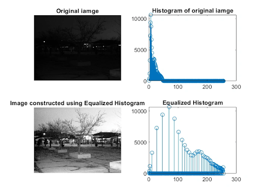
Since different cameras have different color calibration (capture colors differently), we sometimes need to apply histogram equalization or color balancing. It helps the model training process converge (learn) faster.

Handling Missing Data

Handling the missing values often refers to dealing with images that have missing labels in computer vision. Depending on the workflow, we can either remove these images or filter them out and add them to a queue for annotation.

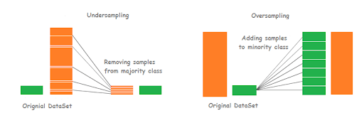
Class Balancing (Oversampling / Undersampling)

If the dataset suffers from class imbalance, we can address this at this stage by applying two techniques: undersampling and oversampling.

Undersampling randomly drops (removes) some examples from the dominant classes. While oversampling, randomly duplicate samples from the minority classes (use augmentation). 

We can also use advanced techniques like SMOTE (Synthetic Minority Over-sampling Technique) that generate synthetic samples instead of duplicating existing ones.

Data Augmentation and Synthesis 

Data augmentation is a way to increase the variety of the training set (making data more diverse) without collecting new images.

It involves applying random or artificial (synthetic) changes to existing images to create new examples. For instance, a picture of a cat remains a cat if it is flipped horizontally, slightly rotated, or in different lighting.

The goal of augmentation is to help the model learn to recognize objects regardless of these changes (teach model invariance). 

Also, well-chosen augmentations can serve as regularization and help AI models generalize better to unseen data. 

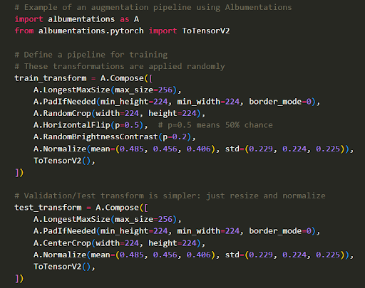
Here are some common types of augmentations and their effects. These can be easily done using libraries like Albumentations or Torchvision.

‍

Here is a sample code to apply augmentation using Albumentations.

Feature Engineering and Representation (Extracting Useful Features)

Feature engineering is the process of selecting, transforming, and combining raw data to create features that improve model performance.

In computer vision, it is about extracting or creating features, such as edges, textures, or shapes, from images (visual data) to help the computer better understand them. 

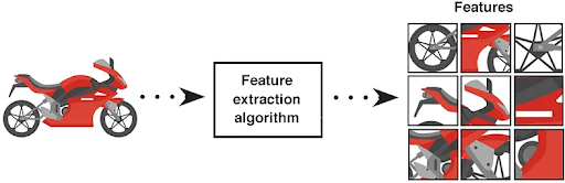
While in traditional approaches, people had to create these features manually, modern deep learning methods have automated much of this process. 

Let's look at both methods in detail.

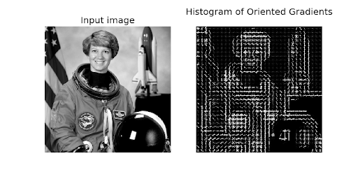
The Classical Approach: Handcrafted Features

In a classic CV, data scientists would spend most of their time manually creating features (handcrafted features). They used complex algorithms to extract descriptive information from images. Common examples include:

• HOG (Histogram of Oriented Gradients): Describes object shapes by capturing the distribution of gradient directions (edge directions).

• SIFT (Scale-Invariant Feature Transform): Identified key points (local features) in an image that were stable across changes in scale, rotation, and lighting.

• Color Histograms: Summarized the color distribution of an image.

These handcrafted features were then fed into a separate model, like a Support Vector Machine (SVM). For instance, in a proof-of-concept with a small dataset, you might extract HOG features from images and train an SVM classifier.

The classical approach still has niche uses, as it is time-intensive and less effective for complex, high-dimensional image data. And now it has been almost entirely replaced in modern computer vision.

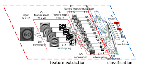
The Modern Approach: Learned Features

In deep learning, Convolutional Neural Networks (CNNs) automatically perform feature engineering and extract features hierarchically through layers of convolution and pooling.

• The first few layers learn to detect simple patterns like edges and corners.
• Middle layers combine these to learn more complex textures and shapes.
• The final layers learn to recognize object parts (like an eye or a wheel) and eventually entire objects.

A very common approach is to start with a pretrained ConvNet (like ResNet, EfficientNet, or a vision transformer) trained on a large dataset. 

We can use this network either as a fixed feature extractor (take outputs from an intermediate layer) or initialize our model’s weights with it. 

Using pretrained models, we can save training time and data, and often yield better features than random initialization.

Dimensionality Reduction

The feature vectors produced by a deep network can be very large, like 2048 dimensions for ResNet50.

Dimensionality reduction techniques like PCA (Principal Component Analysis) can be used to compress these high-dimensional vectors into a smaller, more manageable size while preserving the important information.

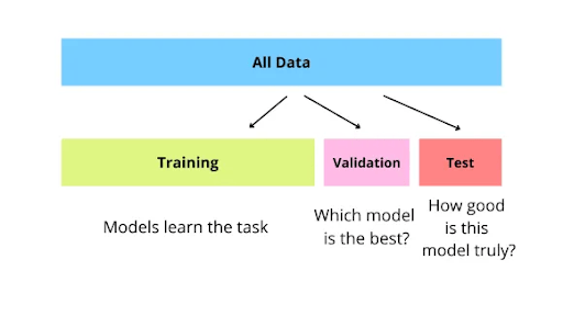
Splitting Data: Training, Validation, and Test Sets 

A simple rule of machine learning is to never evaluate your model on data it has trained on. A model that has memorized the training dataset will get a perfect score, but it will fail when it sees new data.

To prevent this and to get an honest measure of model performance on unseen data, you must split data into (at least) three separate sets (training, validation, and test sets).

• Training Set: This is the largest portion of the data (70–80% of image-label pairs) and is the only set the model learns from. The model sees these image-label pairs during training, updates its weights, and gets better at making predictions.

• Validation Set: A separate hold-out set (10–15% of data) used during development to tune hyperparameters and to make decisions (like when to stop training to avoid overfitting). 

• Test Set: A final, separate set (10–15%) used only once at the end to evaluate (unbiased estimate) how well the model performs on new data.

You can use a simple random split (Scikit-learn’s train_test_split), but in large computer vision datasets, this is not the right approach. 

A random split might fill your sets with thousands of redundant, easy images and miss the rare, important edge cases.

A more organized approach is to curate your splits. You can do this in LightlyStudio with data selection strategies.

For example, for the training set, you can use the DIVERSITY strategies to ensure maximum visual scenarios and reduce redundancy. And you can set a different Number of samples, like 500, 1000, based on your data (70% of your data). 

You can repeat the same approach to create validation and test sets, but use different sampling strategies.

Use the TYPICALITY strategy for a validation set to select a sample (like 10% or 15%) that reflects the overall dataset distribution, and use a different Number of samples.

For the test set (10-15% of data), use the strategy to cover edge cases and challenging examples that test model robustness. 

Also, be sure to exclude the already chosen training images from the new selections. For validation, exclude training images, and for testing, exclude both training and validation images.

With a well-prepared dataset, the pipeline moves to the core stage of model training. Now, let's see how we can pick the right model and train it.

Model Training: Selecting and Training Your Machine Learning Model

The choice of an appropriate machine learning model depends on the specific computer vision task. 

For image classification, CNNs like ResNet, EfficientNet, or MobileNet are common choices. For object detection, models like Faster R-CNN, YOLO (v9 or v12), or SSD are popular. 

For segmentation, U-Net or DeepLab variants are often used. If your task is simpler with small images or a few classes, then a small CNN or classical method (SVM on raw pixels) can work.

Furthermore, when you have limited data, it is best to start from a pretrained model (transfer learning). You can either fine-tune the whole network on your data or freeze early layers and only train the last few layers. 

Transfer learning has its limits, especially when your domain is visually distinct (medical imagery, manufacturing defects, or agricultural data) from the pre-training dataset (ImageNet).

This is where a tool like LightlyTrain comes in. It lets you pretrain a model on your large pool of unlabeled data. It adapts SOTA methods such as DINOv2 or DINOv3 and contrastive learning to your images, creating a domain-specific foundation model. 

In practice, you would run something like:

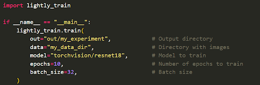
Once done, LightlyTrain saves a checkpoint that has learned meaningful embeddings without using any class information. You can then load the pretrained model and fine-tune it on your labeled data.

LightlyTrain's pretraining whole workflow is a better starting point compared to traditional transfer learning. It leads to significantly higher accuracy (up to 36% mAP increase) during fine-tuning with much less labeled data.

Once you have your model (either from LightlyTrain or a standard pre-trained model), you begin the fine-tuning process. This process involves several key components:

• Batching: The training data is fed to the model in small groups (batches). And the batch size is a key hyperparameter that affects training speed and stability.
• Loss Function: A loss function measures how far the model's prediction is from the true label. For classification, cross-entropy loss is common.
• Optimizer: An optimizer algorithm, like Adam or SGD, updates the model's weights based on the loss function to improve its predictions.
• Training Schedule: This defines the number of epochs (full passes through the training data) and the learning rate schedule.

During training, it is crucial to log metrics like loss and accuracy using tools like TensorBoard or Weights & Biases. This data analysis gives you insight into the model performance. 

Finally, always use version control for your trained model and its corresponding training configuration (date or data version) to ensure reproducibility (consistent results later).

Model Evaluation and Validation (Assessing Model Performance)

After training, you must evaluate your model, which includes computing quantitative metrics and qualitative checks.

Throughout the development cycle, the validation set helps compare different models or hyperparameter settings. The best-performing model on the validation set is usually selected for final testing.

Next, run your model on the test set and compute relevant metrics for your task. Common metrics for vision tasks include:

• Classification: Accuracy, Precision, Recall, F1-Score, and the Confusion Matrix are standard metrics.
• Detection: Mean Average Precision (mAP) is the primary metric, which evaluates both the correctness of the class prediction and the quality of the bounding box localization.
• Segmentation: Mean Intersection over Union (mIoU) is used to measure the overlap between the predicted segmentation mask and the ground truth mask for each class.

Furthermore, conduct error analysis by manually inspecting the samples that the model gets wrong. This qualitative analysis can identify systematic failure modes.

For example, the model might consistently fail on images taken in low-light conditions or on partially occluded objects. These findings offer insights to guide future data collection or model improvements.

Iterative Improvement: Active Learning and Data Feedback Loops

A computer vision pipeline is not a one-time process, but it's an iterative cycle of continuous improvement. 

After the initial model, you might find gaps where the model makes errors. For example, the model may have low confidence or high error on certain image types. You can then target those cases for more data (model-driven data collection).

Instead of randomly labeling more data, you can use active learning within the pipeline. It lets the model pick samples for which it has the highest uncertainty (or that cover underrepresented cases).

These selected samples are prioritized for labeling, creating a human-in-the-loop workflow that directly targets the model's weaknesses.

There are emerging tools and frameworks to support this loop. For example, Lightly AI provides an active learning pipeline that uses embeddings to select diverse, uncertain samples, which can be integrated with labeling tools (LightlyStudio) and retraining.

The following table compares the traditional approach to data labeling with a modern, active learning-enabled pipeline.

‍

Deployment and Monitoring (From Trained Model to Production)

Once your trained model is evaluated and approved, the final step is model deployment. This is how you put your model into a production environment so it can start making predictions on real-world data.

Model Deployment

Deployment involves packaging the trained model and its dependencies into a format (ONNX, TensorFlow SavedModel, or a PyTorch .pt file) that can be served efficiently. 

Common methods include:

• REST or gRPC Service: You can wrap your model in a web server using a tool like FastAPI or Flask. Your application sends an image to the API, and the server runs the model and returns the prediction. For heavier traffic, you can use dedicated model servers like TorchServe or TensorFlow Serving.
• Containers: Another way is to containerize the model using Docker so it can run anywhere (on a cloud server or your own hardware). Since the Docker image includes your model, the inference code, and the necessary libraries. 
• Edge Deployment: For mobile apps or on-device artificial intelligence (like in a car or robot), you can't rely on an internet connection. You must convert the model to a lightweight format like TensorFlow Lite (TFLite) or ONNX and run it directly on the device.
• Cloud Platforms: Services like AWS SageMaker, Google Vertex AI, and Azure ML can manage deployment for you. You upload your model, and they handle creating and scaling the prediction endpoint.

Monitoring in Production

After the deployment, you must continuously monitor the model’s behavior. You can set up logging of predictions and key metrics. 

For example, if you deployed a classifier, log the number of predictions for each class. If you deployed an object detector, log the number of detections or the model's confidence scores.

You can use tools like Prometheus to collect these metrics and Grafana to create dashboards. This helps you watch for real world challenges, like a sudden drop in model performance.

A/B Testing and Rollout

When updating to a new model version, use controlled rollouts (A/B testing). For example, send 90% of traffic to the old model Model A, and 10% to the new one Model B. 

Compare their performance on live data (using ground truth if available, or proxy metrics). Once you are confident the new model is better, you can gradually send more traffic to it.

Feedback to Pipeline

The data from monitoring should feed back into your pipeline. If you notice data drift (when input images change) or drops in performance, consider triggering retraining or active learning. 

Tools and Best Practices for a Successful CV Pipeline

Building a robust computer vision pipeline requires using a combination of tools and libraries, each specialized for a different stage of the machine learning operations workflow

The following table lists recommended tools for building a modern pipeline.

‍

We have outlined the variety of tools, but you need to choose the ones that fit your team’s needs and expertise.

How to Build Better Computer Vision Data Pipelines with Lightly AI

Building and maintaining a visual data pipeline is complex, especially when it comes to the data itself. Lightly's suite of tools is built to solve these data-centric real world challenges in a unified and efficient way.

LightlyEdge (Data Collection at the Source)

LightlyEdge runs directly on your edge devices to collect data from your source and filter redundant images before they ever reach your storage. 

It performs on-device data selection and keeps only diverse and useful samples. By doing this, it reduces bandwidth, lowers storage costs, and streamlines data collection workflow.

LightlyStudio (Dataset Curation, Labeling, and Management)

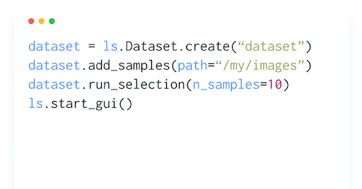
Once you’ve collected data with LightlyEdge, you can upload it to LightlyStudio for curation, annotation, and active data selection. In Python, you can do:

This starts the LightlyStudio UI. It will index all images and compute embeddings. In the UI, you can now see an interactive 2D embedding map of your dataset. 

You can filter images by content or search for similar images by example. Use the built-in label tool to draw boxes or assign classes. 

If you need extra coverage for rare classes or edge cases, you can use Lightly’s AI Data Service to request synthetic images that fill dataset gaps.

LightlyTrain (Model Pretraining and Fine-Tuning)

After curation and labeling, you can use LightlyTrain to pretrain or fine-tune models on curated data. It integrates smoothly with frameworks such as Ultralytics (ultralytics), SuperGradients (super-gradients), TIMM (timm), and RF-DETR (rfdetr).

Below, we provide the minimum scripts for pretraining using ultralytics/yolov12s as an example:

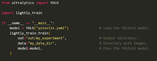
After pretraining, you can load the exported model for fine-tuning with Ultralytics:

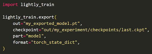
Also, LightlyTrain supports MLflow and Weights & Biases (wandb) for experiment tracking. When ready for deployment (validated), export the model to formats such as ONNX, TorchScript, or TensorRT:

By adopting this workflow, you can label faster and build smarter datasets and models that generalize well.

Conclusion

Building a computer vision machine learning pipeline starts with messy raw data and ends with a model that can be used in real life. It involves cleaning and processing data, training the model, and regularly checking its performance.

By focusing on managing the data carefully, using tools to track changes, automating tasks, and using active learning, you create a system that can grow, adapt, and improve over time. This approach helps build a reliable and scalable system rather than just a one-time trained model.